Atomistic modelling of electronic materials under nonequilibrium conditions

Electronic states and atomic arrangements determine a material's structure, reactions and transport. These six chapters start from the electronic ground state: use DFT to calculate energies, derive forces to follow atomic motion, and search the potential energy surface for reaction pathways and barriers.

Chapter	Central question
I. Overview	How do equilibrium, steady state and nonequilibrium differ? How do electrons and atoms jointly determine material behaviour?
II. DFT and Kohn–Sham Approach	How does electron density determine the ground-state energy, and why is self-consistency necessary?
III. Periodic Systems and Pseudopotential	How does crystal periodicity simplify electronic structure calculations, and how can their cost be reduced?
IV. Structural Phase Changes	How do electronic energies determine atomic forces, motion and structural changes?
V. Thermal Catalysis	How do catalysts activate molecules, alter pathways and lower reaction barriers?
VI. Nudged Elastic Band Method	How are minimum energy paths and transition states located?

I. Overview

Atomistic modelling starts from atomic nuclei and electrons to explain material structures, reactions, and transport. The electron distribution determines the forces on atoms, while atomic positions determine electronic orbitals and energy levels. Understanding how a material changes therefore usually requires connecting its electronic structure to atomic motion.

The first six chapters establish methods for equilibrium electronic structure calculations, then use total energies and forces to study atomic motion, catalysis, and reaction pathways. Two concrete questions illustrate this approach: why do metal clusters become more active for nitrogen reduction when supported on graphene, and why can small atomic displacements in a molecular junction cause a sudden increase in current?

1. Equilibrium, steady state, and nonequilibrium

A steady state has time-independent macroscopic averages:

$$\frac{d\langle A\rangle}{dt}=0.$$

Equilibrium additionally requires the absence of sustained net transport driven by thermodynamic imbalances such as temperature or chemical-potential differences. Connected regions in thermal equilibrium have the same temperature; regions that can exchange the same particle species have the same chemical potential at equilibrium. For charged particles, the transport driving force is described by the electrochemical potential, which includes the effect of the electric potential.

Constant averages do not mean stationary microscopic particles. Particles in an equilibrium gas still move and collide, and their energy distribution depends on momentum. What remains stationary is the statistical distribution. Equilibrium does not imply zero particle momentum or a momentum-independent probability distribution.

Nonequilibrium processes commonly take two forms:

• Time-dependent processes: atomic positions, electronic states, or other averages change with time, as in structural phase transitions, chemical reactions, electronic excitations, and motion under external forces.
• Steady-state transport: the system maintains a steady average density while sustaining mass, charge, spin, or heat transport.

A wire connected to a battery is a nonequilibrium steady state. Electrons continuously pass through it, but equal inflow and outflow rates can keep the local average electron number constant. Similarly, water can flow continuously through a pipe while the amount of water inside stays constant. The initial establishment of current is a transient process; a stable current is a steady state. If the current then displaces contact atoms, the structure begins another time-dependent process.

Both an equilibrium gas in a heat bath and a wire carrying a stable current are therefore steady states, but only the former is also in equilibrium.

2. Statistical ensembles: what can the system exchange with its surroundings?

An ensemble is a collection of microstates and their probabilities under specified macroscopic conditions. To choose an ensemble, first determine whether the system can exchange energy, particles, or neither with its surroundings.

Ensemble	Fixed macroscopic quantities	Exchange with surroundings
Microcanonical	$N,V,E$	Isolated; no energy or particle exchange
Canonical	$N,V,T$	Energy exchange with a heat bath
Grand canonical	$\mu,V,T$	Energy and particle exchange with a reservoir

Microcanonical ensemble

An isolated system has fixed particle number $N$, volume $V$, and energy $E$. If $W$ microstates are accessible, they have equal probabilities:

$$p_i=\frac{1}{W},\qquad \sum_{i=1}^{W}p_i=1.$$

Canonical ensemble

A system in contact with a heat bath has fixed $N,V,T$, but its energy can fluctuate. A microstate of energy $E_i$ is weighted by the Boltzmann factor:

$$p_i=\frac{e^{-\beta E_i}}{Z} =e^{\beta(F-E_i)},\qquad \beta=\frac{1}{k_{\mathrm B}T}.$$

The partition function normalizes the probabilities and determines the Helmholtz free energy:

$$Z=\sum_i e^{-\beta E_i},\qquad F=-k_{\mathrm B}T\ln Z.$$

The probability of an individual microstate differs from the total probability of an energy level. If a level $E$ has degeneracy $g(E)$, its total probability is proportional to $g(E)e^{-\beta E}$. Higher energy reduces the weight of each state, whereas greater degeneracy increases the number of states at that energy.

For example, if two nondegenerate states differ in energy by $2k_{\mathrm B}T$, the ratio of the higher-state probability to the lower-state probability is $e^{-2}\approx0.135$. If these are the only two states, the probability of occupying the higher state is

$$p_{\mathrm{high}}=\frac{e^{-2}}{1+e^{-2}}\approx0.119.$$

Grand canonical ensemble

When a system exchanges both energy and particles with a reservoir, its chemical potential $\mu$, volume $V$, and temperature $T$ are fixed, while its particle number $N$ can fluctuate. The statistical weight is determined by $E-\mu N$:

$$p_{i,N} =\frac{e^{-\beta(E_{i,N}-\mu N)}}{\Xi} =e^{\beta(\Omega+\mu N-E_{i,N})}.$$

The grand partition function and grand potential are

$$\Xi=\sum_N\sum_i e^{-\beta(E_{i,N}-\mu N)},\qquad \Omega=-k_{\mathrm B}T\ln\Xi.$$

All three ensembles calculate averages by weighting physical quantities with their probabilities:

$$\langle A\rangle=\sum_i p_i A_i,$$

The grand canonical ensemble also requires a sum over particle number. These probabilities describe equilibrium statistics; electrons carrying a steady current generally cannot be described by a single equilibrium distribution shared throughout the system.

3. Coupling between electrons and atoms

Electronic materials consist of ions and electrons. Atomic motion changes electronic orbitals and energy levels; electronic redistribution changes interatomic forces. Bond formation and bond breaking therefore involve both electronic rearrangement and atomic motion.

Time-dependent ion motions include structural phase transitions and chemical reactions. Time-dependent electronic properties include electronic excitations and electronic phase transitions. DC electric currents and spin currents describe steady charge and spin transport. Thermoelectric effects connect electrical and thermal transport, as when a temperature difference produces a voltage.

In many problems involving atomic motion, electrons adjust faster than atoms move. One can first determine the electronic state at fixed atomic positions, then differentiate its energy with respect to those positions to obtain forces and follow the structural evolution. Equilibrium electronic ground-state calculations are thus the starting point for potential energy surfaces, molecular dynamics, and reaction-path calculations.

4. Why do metal clusters on graphene activate nitrogen more readily?

The key is that defective graphene and a partially deligated cluster jointly form a nitrogen-activation site. The metal and a defect C atom bind opposite ends of the nitrogen molecule, while metal electrons enter its $\pi^*$ antibonding orbitals, weakening the N–N bond and facilitating subsequent hydrogenation. This mechanism explains the Au–Pt and Au–Pd cluster catalysts studied by Yao et al. (2020).

From a ligand-protected cluster to a nitrogen adsorption site

The intact $\mathrm{Au}_4\mathrm{Pt}_2(\mathrm{SR})_8$ cluster is surrounded by eight sulfur-containing ligands. During anchoring, two $\mathrm{SR}$ ligands at the bottom are removed. The exposed Pt bonds to C atoms at the graphene defect edge, anchoring $\mathrm{Au}_4\mathrm{Pt}_2(\mathrm{SR})_6$ at a divacancy: a defect formed by two missing adjacent C atoms.

Ligand removal also changes the electronic states available for bonding. The energy gap decreases, and singly occupied states derived from Pt $5d$ and Au $6s$ appear. Each contains one electron and lies at relatively high energy, making electron donation to nitrogen easier. The same cluster on defect-free graphene still cannot adsorb $\mathrm N_2$, showing that ligand removal and the defect site must act together.

Adsorbed nitrogen bridges the cluster and the defect C atom. One end forms a C–N bond, while the other forms a metal–N bond with nearby Pt/Au. This two-ended geometry both holds the molecule in place and brings it into contact with C and metal orbitals that can participate in bonding. The proposed local Pt coordination was also assessed by comparing the main peak positions and shapes of simulated and experimental XANES spectra.

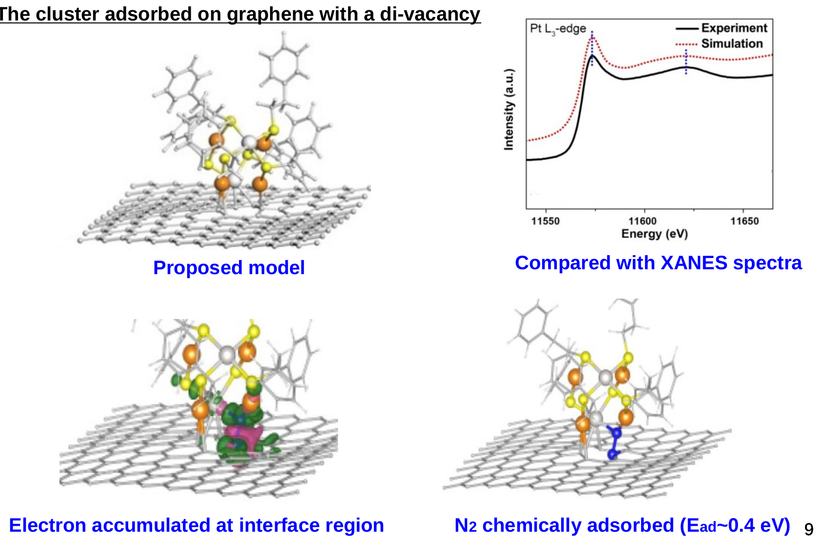
The defect C atom and nearby metal bind opposite ends of nitrogen. Charge-density-difference isosurfaces show electron accumulation and depletion after adsorption; blue atoms mark the nitrogen molecule. The XANES comparison tests the model of local Pt coordination.

Donation, back-donation, and weakening of the N–N bond

After adsorption, nitrogen orbitals mix with metal $d$ orbitals. Electron transfer occurs in both directions: occupied nitrogen $\sigma$ orbitals donate to the metal, and the metal back-donates into nitrogen $\pi^*$ orbitals. Back-donation increases antibonding occupation and weakens the N–N bond. The system's Fermi level and nitrogen LUMO differ by approximately $0.6\,\mathrm{eV}$; Bader analysis gives a net gain of about $1.44$ electrons by nitrogen.

The charge-density difference shows where electrons accumulate or are depleted after adsorption:

$$\Delta\rho(\mathbf r) =\rho_{\mathrm{cat}+\mathrm N_2}(\mathbf r) -\rho_{\mathrm{cat}}(\mathbf r) -\rho_{\mathrm N_2}(\mathbf r).$$

All three densities use the same atomic positions as in the adsorbed geometry. $\Delta\rho>0$ indicates electron accumulation, and $\Delta\rho<0$ indicates depletion. Integration over selected regions or charge partitioning can further estimate transferred electron numbers. This comparison describes electronic rearrangement in the system containing adsorbed nitrogen.

The adsorption energy is defined as

$$E_{\mathrm{ads}} =E_{\mathrm{cat}+\mathrm N_2}-E_{\mathrm{cat}}-E_{\mathrm N_2}.$$

Here, $E_{\mathrm{ads}}=-0.38\,\mathrm{eV}$, so adsorption lowers the energy. Activation does not immediately remove the N–N bond: its occupation and bond strength change first, and successive hydrogenation then converts the two N atoms into ammonia.

Successive hydrogenation, desorption, and energy barriers

The net reaction in an acidic electrolyte is

$$\mathrm N_2+6\mathrm H^++6e^-\longrightarrow2\mathrm{NH}_3.$$

It has the same overall atomic stoichiometry as $\mathrm N_2+3\mathrm H_2\to2\mathrm{NH}_3$, but the electrochemical reduction is supplied jointly by protons and electrons.

This pathway first hydrogenates the N atom attached to graphene. Three H atoms are added successively, and the first ammonia molecule is released. Another three H atoms are then added to the N still attached to the metal, releasing the second ammonia molecule. Product desorption frees the site for another catalytic cycle. The final ammonia desorption requires about $0.91\,\mathrm{eV}$, the largest energy cost along this pathway.

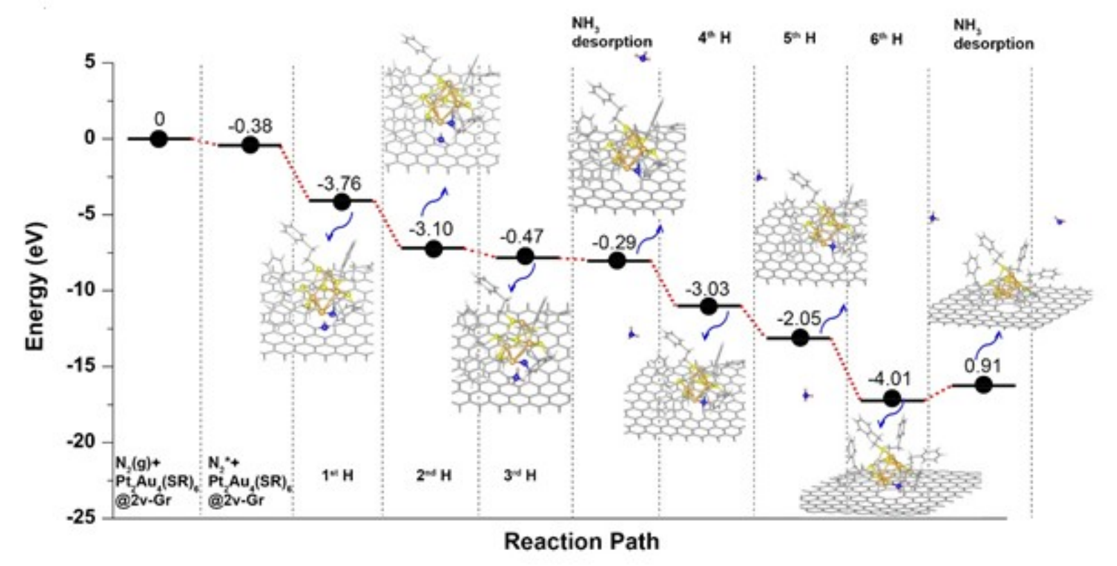
The horizontal axis orders the reaction steps, and the vertical axis gives relative energy. The atomic structures show two successive sequences of hydrogenation and ammonia desorption. Values beside the plateaus are energy changes between consecutive steps; intermediate-state energies and transition-state barriers are different quantities.

When reading reaction energies, distinguish the change between consecutive steps from the energy relative to a common starting point. For example, if adsorption lowers the energy by $0.38\,\mathrm{eV}$ and the next step lowers it by another $3.76\,\mathrm{eV}$, the second plateau lies at $-4.14\,\mathrm{eV}$ relative to the starting point. Comparing states with different numbers of added H atoms also requires including the reference energy of the added hydrogen.

Reaction energy compares the initial and final states. The activation barrier is measured from the preceding energy minimum to the transition state for that step:

$$\Delta E=E_{\mathrm{final}}-E_{\mathrm{initial}},\qquad E_a=E_{\mathrm{TS}}-E_{\mathrm{initial}}.$$

Intermediate-state energies describe the energetic favourability of a reaction, but its rate also depends on the difficulty of reaching the transition state. Even an exothermic step may first have to cross a high barrier.

Production rate and Faradaic efficiency

The experimental comparison uses potentials relative to the reversible hydrogen electrode (RHE), with ammonia production rates normalized by catalyst mass and time. At $-0.1\,\mathrm V$, graphene-supported Pt clusters produce ammonia at approximately three times the rate of unsupported clusters; the Pd system reaches its peak at $-0.2\,\mathrm V$.

More negative potentials also promote the competing hydrogen evolution reaction (HER). The Pd system suppresses HER more effectively, allowing a higher ammonia production rate at a more negative potential. Optimizing the nitrogen reduction reaction (NRR) therefore requires both promoting nitrogen activation and hydrogenation and reducing the fraction of electrons consumed by hydrogen evolution.

Faradaic efficiency measures the fraction of total charge used to produce ammonia:

$$\mathrm{FE}_{\mathrm{NH}_3} =\frac{3F n_{\mathrm{NH}_3}}{Q}.$$

$F$ is the Faraday constant, $n_{\mathrm{NH}_3}$ is the amount of ammonia produced in moles, and $Q$ is the total charge passed. The factor 3 follows from the three electrons required per ammonia molecule. Production rate describes how quickly ammonia is made; FE describes how efficiently electrons are used for that purpose. If the current doubles while the ammonia production rate stays fixed, $Q$ doubles over the same time interval and FE halves.

5. How does bias change the structure and current of a molecular junction?

Bias changes the electron distribution in a molecular junction and therefore changes the forces on its atoms. A structure stable at zero bias may adopt a different configuration when current flows. Wang et al. (2024) studied an oligophenylene-bridged bis-triarylamines junction connected to Au electrodes through S at both ends. The molecule contains five phenyl-ring groups and terminal methyl groups.

The simulations were performed at $300\,\mathrm K$, allowing the molecule and contact Au atoms to move, with a time step of $2\,\mathrm{fs}$. At $1.4\,\mathrm V$, a structural change near the source contact occurred after approximately $100\,\mathrm{fs}$, increasing the average Au–S bond length by about $0.3\,\text{\AA}$. At $1.3\,\mathrm V$, the junction continued to fluctuate around its original configuration.

Bias-dependent energy and atomic forces

The effective energy used in this steady-state density functional theory (SS-DFT) calculation contains a bias-dependent term:

$$\widetilde E=E_{\mathrm{SS}}+E_n,\qquad E_n=-\frac{eV_b}{2}\int\rho_n(\mathbf r)\,d^3r.$$

$V_b$ is the bias, $e>0$ is the elementary charge, and $\rho_n$ is the nonequilibrium electron density. Atomic forces are the negative derivatives of the full effective energy with respect to atomic positions:

$$\mathbf F_I =-\frac{\partial\widetilde E}{\partial\mathbf R_I} =-\frac{\partial E_{\mathrm{SS}}}{\partial\mathbf R_I} -\frac{\partial E_n}{\partial\mathbf R_I}.$$

After the structural change, $E_n$ decreases enough to compensate for an increase in $E_{\mathrm{SS}}$. Electronic effects under bias drive the change while the thermostat maintains $300\,\mathrm K$. The relative effective energies are referenced to the initial configuration at $1.4\,\mathrm V$.

This treatment combines an electronic steady state with time-dependent atomic motion. At each instantaneous geometry, the electrons first establish a steady state; the atoms then move more slowly under the corresponding forces. The two timescales describe different degrees of freedom.

From orbital coupling to transmission and current

In fixed-geometry TranSIESTA and SS-DFT calculations, current increases gradually with bias. SS-DFT calculations that allow structural change instead show a sudden current increase near $1.4\,\mathrm V$. Atomic displacements and group rotations change the overlap between Au $5d$ and S $3p$ orbitals at the source contact, producing additional transmission peaks within the bias window.

For coherent transport, the Landauer formula relates the transmission spectrum to current:

$$I(V)=\frac{2e}{h}\int T(E,V)\left[f_L(E)-f_R(E)\right]dE.$$

$T(E,V)$ is the transmission function, $f_L,f_R$ are the Fermi distributions of the left and right electrodes, and the factor 2 accounts for spin degeneracy. At low temperature, the occupation difference is largest within the bias window between the electrode electrochemical potentials. Transmission changes contribute substantially to net current when they fall within the effective transport window: peaks that grow, broaden, or move into the window can all increase the integral.

Orbital overlap depends on distance, orientation, and symmetry. Group rotation can improve the coupling of relevant orbitals even as the Au–S bond lengthens, so bond length alone does not determine current. The full transmission spectrum determines the Landauer integral. At fixed bias, if $T(E,V)$ doubles throughout the window while electrode distributions remain unchanged, the current doubles too.

6. Learning goals and checks

Understanding atomistic modelling means being able to identify the degrees of freedom being calculated, the approximations used, the inputs and outputs, and how the results explain material behaviour. The first six chapters cover equilibrium electronic structure, periodic systems, atomic motion, thermal catalysis, and reaction pathways. Necessary formulas are provided in the closed-book test, so revision should focus on notation, applicability, calculation steps, and physical meaning.

Use these three questions to check the main ideas:

1. Are time-independent macroscopic averages sufficient to establish equilibrium? No. Check whether temperature or electrochemical-potential differences sustain net transport.
2. Why does graphene enhance activity in the nitrogen reduction system? Defect C and the partially deligated cluster jointly bind nitrogen. Ligand removal creates relatively high-energy occupied states, allowing metal-to-nitrogen $\pi^*$ back-donation that weakens the N–N bond for subsequent hydrogenation.
3. If the initial, transition, and final states have energies $0$, $0.60$, and $-0.40\,\mathrm{eV}$, what are the reaction energy and forward and reverse barriers? They are $-0.40$, $0.60$, and $1.00\,\mathrm{eV}$, respectively. The reaction is exothermic but still has a forward barrier.

II. Equilibrium Modelling: Density Functional Theory and Kohn–Sham Approach

Given the atomic species and positions, electron number, and external conditions, the first task is to calculate the electronic ground-state density and total energy. Comparing total energies for different atomic arrangements reveals their relative stability. Studying how energy changes with atomic positions then gives forces and potential energy surfaces.

Density functional theory (DFT) uses the electron density as its basic variable. The Hohenberg–Kohn theorems explain why density is sufficient to describe the ground state; the Kohn–Sham method provides solvable auxiliary orbital equations; and LDA, GGA, and LSDA approximate the exchange-correlation functional required in practical calculations.

1. From the many-electron wavefunction to electron density

The many-electron problem begins with the Schrödinger equation:

$$\hat H\Psi=E\Psi,\qquad \langle A\rangle=\langle\Psi|\hat A|\Psi\rangle.$$

With nuclear positions fixed, the electronic Hamiltonian is

$$\hat H =-\frac{\hbar^2}{2m_e}\sum_i\nabla_i^2 -\sum_{i,I}\frac{Z_Ie^2}{4\pi\epsilon_0r_{iI}} +\sum_{i<j}\frac{e^2}{4\pi\epsilon_0r_{ij}}.$$

The three terms are electron kinetic energy, electron–nucleus attraction, and electron–electron repulsion. $i,j$ label electrons, $I$ labels nuclei, $Z_I$ is the nuclear charge number, and $i<j$ ensures that each electron pair is counted once. Nuclear repulsion is constant during the electronic solution at fixed nuclear positions; it must be added back when comparing total energies of different structures.

A wavefunction for $N$ electrons depends on $3N$ spatial coordinates as well as spin. The electron density $\rho(\mathbf r)$ depends only on a three-dimensional position and satisfies

$$\rho(\mathbf r)\ge0,\qquad \int\rho(\mathbf r)\,d^3r=N.$$

The true many-electron density is obtained by integrating over the other electrons' coordinates and summing over spin:

$$\rho(\mathbf r) =N\sum_{\sigma_1}\int \left|\Psi(\mathbf r\sigma_1,x_2,\ldots,x_N)\right|^2 \,dx_2\cdots dx_N.$$

$x_j$ includes the position and spin of electron $j$, and $dx_j$ includes the corresponding integration and summation. Density describes the average number of electrons near a point; it is not obtained by treating the many-electron wavefunction as a single three-dimensional function and simply taking its squared modulus.

The first Hohenberg–Kohn theorem

For a fixed electron–electron interaction, the ground-state density determines the external potential $V_{\mathrm{ext}}(\mathbf r)$ up to an additive constant. It therefore determines the Hamiltonian and ground-state properties. Adding a constant to the external potential only shifts the energy zero.

Ground-state observables can be written as functionals of the density:

$$\langle A\rangle=A[\rho].$$

A functional maps a function to a number: its input is an entire density distribution, and its output is a number. The theorem establishes that density contains sufficient information, but does not supply the explicit energy functional.

The second Hohenberg–Kohn theorem and the variational principle

The electronic energy is written as

$$E[\rho]=F_{\mathrm{HK}}[\rho] +\int\rho(\mathbf r)V_{\mathrm{ext}}(\mathbf r)\,d^3r, \qquad F_{\mathrm{HK}}[\rho]=T[\rho]+V_{ee}[\rho].$$

$T$ is the true many-electron kinetic energy, and $V_{ee}$ is the electron interaction energy. $F_{\mathrm{HK}}$ is a universal functional: for a fixed electron interaction, it does not depend on the external potential of a particular material. The atomic configuration enters through $V_{\mathrm{ext}}$.

At fixed external potential and electron number, the ground-state density minimizes the energy:

$$E_0=\min_{\rho\to N}E[\rho],\qquad E[\widetilde\rho]\ge E_0.$$

An admissible trial density must be nonnegative, integrate to $N$, and arise from a valid many-electron state. The conventional variational method minimizes $\langle\Psi|\hat H|\Psi\rangle$ over normalized wavefunctions, whereas DFT minimizes $E[\rho]$ over admissible densities. Both seek the same ground state.

This comparison concerns different trial densities evaluated with the same exact functional. If two approximate functionals give $-10$ and $-11\,\mathrm{eV}$, the lower value alone does not establish greater accuracy.

2. Hartree energy and the Kohn–Sham auxiliary system

From this point onward, atomic units are used: $\hbar=m_e=e=4\pi\epsilon_0=1$. The external-potential energy can be evaluated directly by integrating the density. The classical part of the electron–electron interaction is the Hartree energy:

$$E_H[\rho]=J[\rho] =\frac12\iint \frac{\rho(\mathbf r)\rho(\mathbf r')}{|\mathbf r-\mathbf r'|} \,d^3r\,d^3r'.$$

It treats electrons as a continuous charge cloud. The double integral counts both $(\mathbf r,\mathbf r')$ and $(\mathbf r',\mathbf r)$, so the factor $1/2$ avoids double counting.

The Hartree mean field does not fully include exchange and correlation. Exchange arises from the antisymmetry of a fermionic wavefunction; correlation describes correlated electron motion beyond an independent-particle approximation. The true kinetic energy $T[\rho]$ is also difficult to express directly as a simple density functional.

Calculating kinetic energy from auxiliary orbitals

The Kohn–Sham method constructs an auxiliary system of noninteracting electrons with the same ground-state density as the real system. Its wavefunction can be represented by a Slater determinant:

$$\Phi_s=\frac{1}{\sqrt{N!}}\det[\varphi_i(x_j)].$$

Exchanging two electrons changes the determinant's sign, automatically satisfying the Pauli principle. Each occupied spin orbital holds at most one electron. With $f_i$ denoting the occupation number, the density and auxiliary kinetic energy are

$$\rho(\mathbf r)=\sum_i f_i|\varphi_i(\mathbf r)|^2, \qquad T_s=\sum_i f_i \left\langle\varphi_i\left|-\frac12\nabla^2\right|\varphi_i\right\rangle.$$

For spin-degenerate spatial orbitals, double occupation corresponds to $f_i=2$; for separately represented spin orbitals, occupation cannot exceed 1. The true wavefunction and auxiliary Slater determinant may differ, but their electron densities must agree.

The exact exchange-correlation decomposition

The Kohn–Sham total energy is written as

$$E[\rho]=T_s[\rho] +\int\rho V_{\mathrm{ext}}\,d^3r +E_H[\rho]+E_{\mathrm{xc}}[\rho],$$

where

$$E_{\mathrm{xc}}[\rho] =\bigl(T[\rho]-T_s[\rho]\bigr) +\bigl(V_{ee}[\rho]-E_H[\rho]\bigr).$$

Thus, $T_s$ is not equal to the true kinetic energy $T$. The kinetic-energy difference $T-T_s$ is included in $E_{\mathrm{xc}}$ together with the nonclassical interaction energy. Given the exact $E_{\mathrm{xc}}$, this decomposition is itself exact. Practical calculations usually introduce an approximation when selecting the exchange-correlation functional.

For example, if $T=12,T_s=10,V_{ee}=8,E_H=9$ in consistent energy units, then $E_{\mathrm{xc}}=(12-10)+(8-9)=1$. Calculating only $V_{ee}-E_H=-1$ would omit the kinetic-energy difference.

3. Deriving the Kohn–Sham equations variationally

The auxiliary orbitals satisfy orthonormality:

$$\int\varphi_i^*(\mathbf r)\varphi_j(\mathbf r)\,d^3r=\delta_{ij}.$$

Each orbital is normalized, and distinct orbitals are orthogonal. The complex conjugate must be retained for general complex orbitals. For this derivation, take the occupation of each occupied spin orbital to be 1 and impose these conditions using Lagrange multipliers:

$$\mathcal L =E-\sum_{ij}\epsilon_{ij} \left(\int\varphi_i^*\varphi_j\,d^3r-\delta_{ij}\right), \qquad \frac{\delta\mathcal L}{\delta\varphi_i^*}=0.$$

Variation of the kinetic energy with respect to an orbital gives $-\tfrac12\nabla^2\varphi_i$; the density dependence of the remaining energy terms produces the effective potential. Diagonalizing the multiplier matrix $\epsilon_{ij}$ gives the Kohn–Sham equation in single-electron form:

$$\left[-\frac12\nabla^2+V_{\mathrm{eff}}(\mathbf r)\right] \varphi_i(\mathbf r)=\epsilon_i\varphi_i(\mathbf r),$$

$$V_{\mathrm{eff}}=V_{\mathrm{ext}}+V_H+V_{\mathrm{xc}},$$

$$V_H(\mathbf r) =\int\frac{\rho(\mathbf r')}{|\mathbf r-\mathbf r'|}\,d^3r', \qquad V_{\mathrm{xc}}(\mathbf r) =\frac{\delta E_{\mathrm{xc}}}{\delta\rho(\mathbf r)}.$$

The Hartree potential has no factor $1/2$: varying $E_H$ produces one contribution from each density factor, cancelling that coefficient. The meaning of a functional derivative can be expressed as

$$\delta E_{\mathrm{xc}} =\int V_{\mathrm{xc}}(\mathbf r)\,\delta\rho(\mathbf r)\,d^3r,$$

which gives the first-order exchange-correlation energy change caused by a small density variation.

Although these equations have a single-electron form, the effective potential still depends on the total density produced by all occupied orbitals. The total energy also includes corrections to the counting of interactions, so it cannot simply be replaced by the eigenvalue sum $\sum_i f_i\epsilon_i$.

4. Self-consistent field: matching the input and output densities

The Kohn–Sham solution is circular: density determines the potential, the potential determines the orbitals, and the orbitals produce a new density. A self-consistent field (SCF) calculation proceeds as follows:

1. Choose an initial density that integrates to $N$, denoted by $\rho_{\mathrm{in}}$.
2. Use it to construct $V_H$ and $V_{\mathrm{xc}}$, then combine them with the known external potential to obtain $V_{\mathrm{eff}}$.
3. Solve the Kohn–Sham eigenvalue equations and determine orbital occupations from the electron number.
4. Calculate $\rho_{\mathrm{out}}=\sum_i f_i|\varphi_i|^2$ from the orbitals.
5. Compare the input and output densities and check the energy change. If convergence has not been reached, update the input and repeat.

The self-consistency condition is

$$\rho_{\mathrm{out}}[\rho_{\mathrm{in}}]=\rho_{\mathrm{in}}.$$

A single eigenvalue solution only gives orbitals in the current potential. Self-consistency requires the density produced by those orbitals to match the density used to construct that potential. Numerically, the density difference and energy change must fall below specified tolerances.

Replacing the input entirely with the new density can cause oscillations. Simple density mixing combines the old and new densities:

$$\rho_{\mathrm{in}}^{(n+1)} =(1-\alpha)\rho_{\mathrm{in}}^{(n)} +\alpha\rho_{\mathrm{out}}^{(n)}, \qquad 0<\alpha\le1.$$

A smaller $\alpha$ gives a more conservative update. For example, if the input and output densities at a point are $0.80$ and $1.20$, with $\alpha=0.25$, the next input is $0.75\times0.80+0.25\times1.20=0.90$. If both density distributions integrate to $N$, their mixture preserves the total electron number.

5. LDA: using a uniform electron gas locally

The local density approximation (LDA) estimates the exchange-correlation energy per electron at each point using a uniform electron gas of the same density, then multiplies by the local density and integrates over space:

$$E_{\mathrm{xc}}^{\mathrm{LDA}}[\rho] =\int\rho(\mathbf r)\,\epsilon_{\mathrm{xc}}(\rho(\mathbf r))\,d^3r.$$

$\epsilon_{\mathrm{xc}}$ is an energy per electron, whereas $\rho\epsilon_{\mathrm{xc}}$ is an energy per unit volume. The material's density may still vary spatially; "local" means that the energy at each point uses only the density value at that point.

Because the density dependence is local, the functional derivative reduces to an ordinary derivative:

$$V_{\mathrm{xc}}^{\mathrm{LDA}} =\frac{d[\rho\epsilon_{\mathrm{xc}}(\rho)]}{d\rho} =\epsilon_{\mathrm{xc}}+\rho\frac{d\epsilon_{\mathrm{xc}}}{d\rho}.$$

The first term comes from the density prefactor, and the second from the density dependence of the energy per electron. The potential requires differentiating the whole product. For example,

$$\epsilon_{\mathrm x}=-C\rho^{1/3} \quad\Longrightarrow\quad E_{\mathrm x}=-C\int\rho^{4/3}\,d^3r, \qquad V_{\mathrm x}=-\frac{4C}{3}\rho^{1/3}.$$

6. GGA and BLYP: including spatial density variations

Two points can have the same density but different rates of variation in their surroundings. The generalized gradient approximation (GGA) also uses the density gradient as an input:

$$E_{\mathrm{xc}}^{\mathrm{GGA}}[\rho] =\int\rho(\mathbf r)\,\epsilon_{\mathrm{xc}}(\rho,\nabla\rho)\,d^3r, \qquad E_{\mathrm{xc}}=E_{\mathrm x}+E_{\mathrm c}.$$

$\nabla\rho$ describes the direction and rate of density variation. Exchange and correlation can still be calculated separately and added. BLYP combines Becke exchange with Lee–Yang–Parr correlation; PBE is the Perdew–Burke–Ernzerhof functional. Changing the functional changes the exchange-correlation energy and potential, while the Kohn–Sham equations and SCF procedure remain the same.

Why does the GGA potential contain a divergence term?

Writing $E_{\mathrm{xc}}=\int g(\rho,\nabla\rho)\,d^3r$, a variation in density also changes its gradient:

$$\delta E_{\mathrm{xc}} =\int\left[ \frac{\partial g}{\partial\rho}\,\delta\rho +\frac{\partial g}{\partial(\nabla\rho)}\cdot\nabla\delta\rho \right]d^3r.$$

Integrating the second term by parts and taking the boundary term to vanish gives

$$V_{\mathrm{xc}} =\frac{\partial g}{\partial\rho} -\nabla\cdot\frac{\partial g}{\partial(\nabla\rho)}.$$

The first term is the contribution from changing the density directly; the second comes from changing its gradient. Differentiating only the explicit $\rho$ dependence would miss the second contribution.

Local exchange, gradient corrections, and correlation in BLYP

Using the dimensionless relative density gradient

$$x=\frac{|\nabla\rho|}{\rho^{4/3}},$$

the Becke exchange form used in this course is

$$E_{\mathrm x} =-\int C_{\mathrm x}\rho^{4/3}\,d^3r -\int b\rho^{4/3} \frac{x^2}{1+6bx\operatorname{arsinh}(x)}\,d^3r.$$

$C_{\mathrm x}$ and $b$ are parameters. The first term is local exchange, and the second is the gradient correction. For a uniform density, $\nabla\rho=0$, so $x=0$; the correction vanishes and local exchange is recovered. Here $\sinh^{-1}(x)$ means the inverse hyperbolic sine, $\operatorname{arsinh}(x)$, which differs from $1/\sinh(x)$.

LYP correlation uses the density, its derivatives, an auxiliary quantity $t(\mathbf r)$, and parameters $a,b,c,d$ to describe correlation in a nonuniform electron distribution. The Laplacian $\nabla^2\rho$ describes local density curvature. The correlation potential used in self-consistent calculations is still obtained from $V_{\mathrm c}=\delta E_{\mathrm c}/\delta\rho$; correlation energy itself is not a potential.

7. Spin-DFT: solving for both spin channels

Magnetic systems require separate spin-up and spin-down densities. Here the collinear-spin description defines both channels along a common quantization axis.

$$\rho=\rho_\uparrow+\rho_\downarrow,\qquad \rho_\sigma(\mathbf r) =\sum_i f_{i\sigma}|\varphi_{i\sigma}(\mathbf r)|^2, \qquad \sigma=\uparrow,\downarrow.$$

Each channel satisfies

$$\left[-\frac12\nabla^2+V_{\mathrm{eff},\sigma}(\mathbf r)\right] \varphi_{i\sigma} =\epsilon_{i\sigma}\varphi_{i\sigma},$$

$$V_{\mathrm{eff},\sigma} =V_{\mathrm{ext},\sigma} +V_H[\rho_\uparrow+\rho_\downarrow] +\frac{\delta E_{\mathrm{xc}}[\rho_\uparrow,\rho_\downarrow]}{\delta\rho_\sigma}.$$

Both channels share the Hartree potential generated by the total charge density. The exchange-correlation potentials depend on how electrons are distributed between the spin channels. Updating one channel therefore affects the other through the effective potentials, so both densities must be iterated together.

Electron number, spin imbalance, and Zeeman energy

Define

$$N_\sigma=\int\rho_\sigma\,d^3r,\qquad M_z=\mu_{\mathrm B}(N_\uparrow-N_\downarrow) =\mu_{\mathrm B}\int(\rho_\uparrow-\rho_\downarrow)\,d^3r.$$

$\mu_{\mathrm B}$ is the Bohr magneton. Here $M_z$ follows the convention based on the difference in spin populations; an electron's physical spin magnetic moment points opposite to its spin. If $N_\uparrow=6,N_\downarrow=4$, then $N=10,M_z=2\mu_{\mathrm B}$. If each channel contains 5 electrons, the integrated spin imbalance vanishes, but positive and negative local spin polarizations may still cancel in the integral.

For a magnetic field along $z$, with $\hat S_z$ eigenvalues taken as $\pm1/2$, the Hamiltonian including the Zeeman term is

$$\hat H =\hat T+\hat V_{ee}+\hat V_{\mathrm{ext}} +2\mu_{\mathrm B}B\sum_i\hat S_{zi}.$$

The single-electron energies in the up and down channels shift by $+\mu_{\mathrm B}B$ and $-\mu_{\mathrm B}B$, respectively. Their total contribution is $+BM_z$ under the convention above:

$$\langle\hat V_{\mathrm{ext}}^B\rangle =\int\rho V_{\mathrm{ext}}\,d^3r+BM_z.$$

Without a spin-dependent external field, both channels use the same external potential. With a Zeeman term, each channel receives the magnetic-field potential with the appropriate sign.

Energy and self-consistency in a spin-polarized system

The energy is decomposed as

$$E=T_s[\rho_\uparrow,\rho_\downarrow] +E_{\mathrm{ext}}+E_H[\rho] +E_{\mathrm{xc}}[\rho_\uparrow,\rho_\downarrow],$$

$$T_s=\sum_{\sigma=\uparrow,\downarrow}\sum_i f_{i\sigma} \left\langle\varphi_{i\sigma}\left|-\frac12\nabla^2\right|\varphi_{i\sigma}\right\rangle.$$

Hartree energy depends only on total density: two spin distributions with the same total density have the same $E_H$. Kinetic and exchange-correlation energies also depend on spin occupation. Exchange depends on same-spin occupations, and correlation also depends on the spin distribution. $E_{\mathrm{xc}}$ retains both spin densities as inputs and includes the difference between the true and auxiliary kinetic energies.

A spin-dependent SCF calculation starts from two initial densities, constructs two potentials, solves for two sets of orbitals, and updates both densities. Convergence must be checked for both charge and spin density: equal and opposite changes in the two channels leave total charge unchanged while changing spin polarization. Different initial magnetizations may converge to different self-consistent magnetic states. To determine the stable state, compare their total energies under the same conditions.

8. LSDA and spin-polarization interpolation

The local spin density approximation (LSDA) uses a uniform electron gas with the same total density and spin distribution at each point:

$$E_{\mathrm{xc}}^{\mathrm{LSDA}}[\rho_\uparrow,\rho_\downarrow] =\int\rho\,\epsilon_{\mathrm{xc}}(\rho_\uparrow,\rho_\downarrow)\,d^3r, \qquad \rho=\rho_\uparrow+\rho_\downarrow.$$

Take a functional derivative with respect to each channel separately:

$$V_{\mathrm{xc},\uparrow} =\epsilon_{\mathrm{xc}} +\rho\frac{\partial\epsilon_{\mathrm{xc}}}{\partial\rho_\uparrow}, \qquad V_{\mathrm{xc},\downarrow} =\epsilon_{\mathrm{xc}} +\rho\frac{\partial\epsilon_{\mathrm{xc}}}{\partial\rho_\downarrow}.$$

When differentiating with respect to $\rho_\uparrow$, hold $\rho_\downarrow$ fixed, so $\partial\rho/\partial\rho_\uparrow=1$. Differentiating the total-density prefactor produces the first term; differentiating the energy per electron produces the second. The other spin density is held fixed, while total density changes with the channel being varied. The down-spin derivation is analogous, and the two potentials can differ.

For example, starting from

$$E_{\mathrm x}=-C\int \left(\rho_\uparrow^{4/3}+\rho_\downarrow^{4/3}\right)d^3r$$

the up-spin exchange potential is

$$V_{\mathrm x,\uparrow} =-\frac{4C}{3}\rho_\uparrow^{1/3}.$$

Representing both channels by total density and spin polarization

Spin polarization is defined as

$$\xi=\frac{\rho_\uparrow-\rho_\downarrow}{\rho_\uparrow+\rho_\downarrow}, \qquad -1\le\xi\le1.$$

Hence,

$$\rho_\uparrow=\frac{\rho}{2}(1+\xi),\qquad \rho_\downarrow=\frac{\rho}{2}(1-\xi).$$

$\xi$ is a local quantity: $\xi=0$ means equal spin densities, while $\xi=1$ and $-1$ represent complete up-spin and down-spin polarization, respectively. At the same total density, one can interpolate between unpolarized and fully polarized uniform electron gases:

$$\epsilon_{\mathrm{xc}}(\rho,\xi) =\epsilon_{\mathrm{xc}}(\rho,0) +\left[\epsilon_{\mathrm{xc}}(\rho,1)-\epsilon_{\mathrm{xc}}(\rho,0)\right]f(\xi),$$

$$f(\xi) =\frac{(1+\xi)^{4/3}+(1-\xi)^{4/3}-2}{2^{4/3}-2}.$$

The denominator gives unit weight at full polarization. Interchanging spin-up and spin-down only changes the sign of $\xi$, so

$$f(0)=0,\qquad f(1)=f(-1)=1,\qquad f(\xi)=f(-\xi).$$

For example, if $\rho_\uparrow=0.06,\rho_\downarrow=0.02$, then $\rho=0.08,\xi=0.5$. If the endpoint exchange-correlation energies per electron at this same total density are $-0.50$ and $-0.60$, then

$$f(0.5)\approx0.219,\qquad \epsilon_{\mathrm{xc}}(\rho,0.5) =-0.50-0.10\times0.219\approx-0.522.$$

The interpolation weight is $f(\xi)$, not simply $\xi$.

9. Three questions to answer before calculating

1. Why is one solution of the Kohn–Sham eigenvalue equations insufficient? The effective potential comes from the input density, while the orbitals generate the output density. Self-consistency requires the two to agree.
2. Why is $E_{\mathrm{xc}}$ more than $V_{ee}-E_H$? Once the auxiliary kinetic energy $T_s$ is used, the true kinetic-energy difference $T-T_s$ must also be included.
3. If total charge density has stopped changing, is spin-DFT necessarily converged? No. The two channels may change in opposite directions while preserving total density. Spin density and energy must also be checked.

III. Periodic Systems and Pseudopotential

1. Kohn–Sham calculations for periodic systems

A crystal calculation still begins with the electronic ground state at fixed atomic positions. Hohenberg–Kohn theory expresses this as a variational problem in the density: hold the external potential and electron number fixed, and find the admissible density that minimizes the energy.

$$E[\rho]=\int V_{\mathrm{ext}}(\mathbf r)\rho(\mathbf r)\,d\mathbf r+F_{\mathrm{HK}}[\rho], \qquad \int\rho(\mathbf r)\,d\mathbf r=N_e.$$

$F_{\mathrm{HK}}$ contains the true electronic kinetic energy and electron–electron interactions; the atomic species and arrangement enter through the external potential $V_{\mathrm{ext}}$. The Kohn–Sham method uses auxiliary one-electron orbitals to calculate the auxiliary system's kinetic energy, placing the remaining contributions in the exchange-correlation functional. In atomic units, the equations are

$$\left[-\frac12\nabla^2+V_{\mathrm{eff}}(\mathbf r)\right]\varphi_i(\mathbf r) =\varepsilon_i\varphi_i(\mathbf r),$$

$$V_{\mathrm{eff}}=V_{\mathrm{ext}}+V_{\mathrm H}+V_{\mathrm{xc}}, \qquad \rho(\mathbf r)=\sum_i f_i|\varphi_i(\mathbf r)|^2.$$

$f_i$ is the occupation number. The Hartree potential describes the classical Coulomb interaction of the electron density, while the exchange-correlation potential accounts for quantum effects missing from this mean-field description. The potential depends on the density, and the occupied orbitals of that potential produce the density. A self-consistent calculation is therefore required: guess the density, construct the potential, solve for the orbitals, and update the density until input and output agree.

$\varepsilon_i$ is an auxiliary orbital eigenvalue. The total energy also includes interaction double-counting corrections, so it cannot simply be replaced by the sum of occupied eigenvalues. For a crystal, the next step is to use the periodicity of the self-consistent potential to reduce the infinite system to calculations within a primitive cell.

2. Bloch's theorem: phase changes between cells

Consider a one-dimensional potential with period $a$, and define the translation operator by

$$V(x+ma)=V(x),\qquad \hat T(a)\psi(x)=\psi(x+a),\qquad m\in\mathbb Z.$$

A rigid translation leaves the kinetic energy unchanged, and a lattice translation also leaves the potential unchanged. Thus,

$$[\hat H,\hat T(a)]=0.$$

The Hamiltonian and translation operator can have simultaneous eigenstates. When degeneracies occur, suitable linear combinations can be chosen within each degenerate subspace. Translation preserves the norm, so its eigenvalues have unit magnitude and can be written as phase factors:

$$\hat T(a)\psi_k=\lambda\psi_k, \qquad |\lambda|=1, \qquad \lambda=e^{ika}.$$

Translation through $m$ cells gives

$$\psi_k(x+ma)=e^{ikma}\psi_k(x).$$

$k$ is the wave vector, with dimensions of inverse length; $\hbar k$ is called crystal momentum. In a periodic potential, crystal momentum generally differs from the mechanical momentum of a free particle.

Define $u_{nk}(x)=e^{-ikx}\psi_{nk}(x)$ and substitute the translation relation to obtain the Bloch form:

$$\psi_{nk}(x)=e^{ikx}u_{nk}(x), \qquad u_{nk}(x+ma)=u_{nk}(x).$$

A Bloch state is a plane wave multiplied by a lattice-periodic function. The plane wave records the phase between cells, while the periodic function describes the electronic distribution within a cell. $n$ labels the bands, and a single $k$ can correspond to several energy eigenstates. Since $u_{nk}$ is generally not constant, a Bloch wave is not simply a free-electron plane wave.

For example, when $k=\pi/(2a)$, translation through one cell gives $i\psi(x)$, two cells give $-\psi(x)$, and four cells restore the original phase. Yet each cell translation satisfies

$$|\psi(x+a)|^2=|\psi(x)|^2.$$

The wavefunction's phase can change while the probability density retains period $a$. Calculating one primitive cell also does not make it an isolated molecule: all translated copies remain connected through the Bloch boundary phase.

3. Reciprocal lattice vectors and the one-dimensional Brillouin zone

If two wave vectors differ by

$$G=\frac{2\pi m}{a},$$

then

$$e^{i(k+G)a}=e^{ika}.$$

$G$ is a reciprocal lattice vector. $k$ and $k+G$ give the same phase under every lattice translation, so they can label the same physical state. Relabeling also requires changing the periodic part:

$$u_{n,k+G}(x)=e^{-iGx}u_{nk}(x), \qquad \psi_{n,k+G}(x)=\psi_{nk}(x).$$

The periodic part cancels the additional plane-wave factor. The energy spectrum therefore has reciprocal-lattice periodicity:

$$E_n(k+G)=E_n(k).$$

A nonredundant set of wave vectors can consequently be placed in an interval of width $2\pi/a$. The usual first Brillouin zone (first BZ) is

$$-\frac{\pi}{a}\leq k<\frac{\pi}{a}.$$

The endpoints are equivalent, so a half-open interval avoids double counting. A longer real-space period gives a narrower reciprocal-space interval. When a supercell is used, the bands fold into its smaller BZ; this is called band folding.

For example, if $a=0.40\,\mathrm{nm}$, then $G_0=15.708\,\mathrm{nm}^{-1}$ and the first BZ is $[-7.854,7.854)\,\mathrm{nm}^{-1}$. Taking $k=12.0\,\mathrm{nm}^{-1}$ and subtracting $G_0$ gives the equivalent wave vector $k'=-3.708\,\mathrm{nm}^{-1}$. Folding adds or subtracts reciprocal lattice vectors. Taking the absolute value instead replaces $k$ by $-k$, which is generally a different state.

4. Three-dimensional lattices, reciprocal space, and primitive cells

An arbitrary translation of a three-dimensional lattice is

$$\mathbf R=m_1\mathbf a_1+m_2\mathbf a_2+m_3\mathbf a_3, \qquad m_i\in\mathbb Z.$$

The primitive real-space vectors $\mathbf a_i$ and reciprocal lattice vectors $\mathbf b_j$ satisfy

$$\mathbf a_i\cdot\mathbf b_j=2\pi\delta_{ij}.$$

An arbitrary reciprocal lattice vector is $\mathbf G=\sum_j h_j\mathbf b_j$, where $h_j$ are integers. Hence,

$$e^{i\mathbf G\cdot\mathbf R}=1,$$

and the Bloch form becomes

$$\psi_{n\mathbf k}(\mathbf r) =e^{i\mathbf k\cdot\mathbf r}u_{n\mathbf k}(\mathbf r), \qquad u_{n\mathbf k}(\mathbf r+\mathbf R)=u_{n\mathbf k}(\mathbf r).$$

$\mathbf k$ and $\mathbf k+\mathbf G$ remain equivalent labels. The first Brillouin zone is the reciprocal lattice's Wigner–Seitz primitive cell. To construct it, connect the reciprocal-space origin to neighboring lattice points, draw the perpendicular bisector planes of these connections, and take the innermost enclosed region containing the origin. Points inside this region are closer to the origin than to any other reciprocal lattice point.

For a simple cubic lattice with side length $a$, the reciprocal basis vectors have length $2\pi/a$. The first BZ is a cube whose components satisfy $-\pi/a\leq k_\alpha<\pi/a$. Other lattices give different polyhedra: the reciprocal lattice determines the BZ shape.

The Bravais lattice describes translations, while the basis specifies the atoms attached to each lattice point. A primitive cell can contain several atoms without increasing the lattice period. Bloch's theorem restricts the calculation of each $u_{n\mathbf k}$ to one primitive cell, but solutions and integration over different $\mathbf k$ are still required.

5. Graphene: relating atomic structure to bands

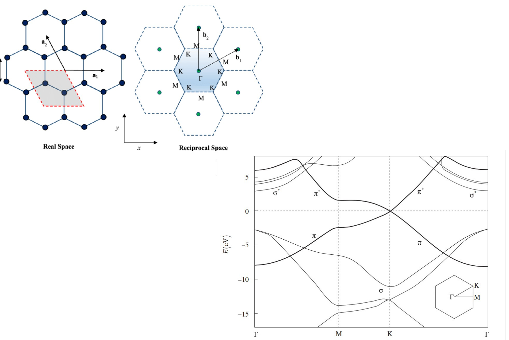
Graphene's honeycomb structure consists of a two-dimensional triangular Bravais lattice with a two-carbon basis. Its primitive cell is the parallelogram spanned by two primitive translation vectors and contains two carbon atoms after accounting for shared boundaries. If the carbon–carbon bond length is $d$, the primitive lattice vectors have length $\sqrt3\,d$. The bond length and lattice constant should be distinguished.

The first BZ is a hexagon in reciprocal space. $\Gamma$ lies at its center, $M$ at an edge midpoint, and $K$ and $K'$ at alternating corners. The carbon hexagons in real space and the BZ in reciprocal space belong to different spaces.

Bands are commonly plotted along high-symmetry paths such as $\Gamma-M-K-\Gamma$. The vertical axis is electronic energy, the horizontal axis follows the wave-vector path, and each curve is a band $E_n(\mathbf k)$. Such paths make the bands easy to inspect, but they cannot replace integration over the full BZ when calculating the electron density.

The $\pi$ states mainly arise from $p_z$ orbitals perpendicular to the plane, while the $\sigma$ bands mainly describe in-plane bonding. An asterisk denotes antibonding character. In ideal graphene, the $\pi$ and $\pi^*$ bands meet near the $K$ points, giving a zero band gap. Their approximately linear dispersion near the touching points forms a Dirac cone.

The valence and conduction bands of ideal graphene meet at the K points. This contact occurs at particular wave vectors. Substrates, defects, or structural changes that break the relevant symmetry can alter the bands and require a calculation for the modified structure. The horizontal axis is also not time: electronic energy as a function of wave vector cannot be read as an atomic trajectory.

6. Frozen-core approximation: retaining the core's influence

Core electrons lie close to the nucleus and are tightly bound; valence electrons participate more readily in bonding and charge transfer. The frozen-core approximation holds the shapes of the core orbitals approximately fixed while allowing the valence electrons to change explicitly. The nucleus and frozen core form an effective ionic core, whose charge screening remains part of the potential experienced by the valence electrons.

If the nuclear charge number is $Z$ and the number of frozen core electrons is $N_{\mathrm{core}}$, then

$$Z_{\mathrm{val}}=Z-N_{\mathrm{core}}.$$

For example, carbon has nuclear charge $+6e$. Freezing the two $1s^2$ electrons leaves an effective ionic core with long-range net charge $+4e$ and four explicit valence electrons. Two neutral carbon atoms therefore require eight valence electrons to be treated explicitly. The effective description changes; the nucleus remains a carbon nucleus.

The valence electrons still move in the complete effective potential:

$$V_{\mathrm{KS}}(\mathbf r) =V_{\mathrm{ext}}(\mathbf r) +V_{\mathrm H}[\rho](\mathbf r) +V_{\mathrm{xc}}[\rho](\mathbf r),$$

$$V_{\mathrm H}[\rho](\mathbf r) =\int\frac{\rho(\mathbf r')}{|\mathbf r-\mathbf r'|}\,d\mathbf r'.$$

A specific LDA or GGA scheme is chosen for exchange and correlation. If semicore states contribute appreciably to bonding, or high pressure causes core regions to overlap, more electrons should be treated as valence electrons. Freezing the core reduces the number of explicit electrons; pseudopotentials further reduce the cost of representing their valence orbitals.

7. Pseudopotentials: smoothing the core region

Near a nucleus, the true valence wavefunction feels a strong nuclear potential and must remain orthogonal to the core states. It therefore has rapid oscillations and multiple nodes. A plane-wave expansion needs short-wavelength, high-wave-vector components to represent these details, making the calculation expensive.

A pseudopotential replaces the true valence wavefunction in the core region with a smooth pseudo wavefunction. Outside the core cutoff radius $r_c$, the required matching is retained:

$$\psi^{\mathrm{PS}}(r)\simeq\psi^{\mathrm{AE}}(r), \qquad r\geq r_c.$$

Smoothing the potential and wavefunction inside the core reduces the required high-wave-vector components. An accurate pseudopotential must also preserve bonding information outside the core and scattering properties over the relevant energy range. Here, softening means smoother spatial variation.

Common approaches include:

• Norm-conserving pseudopotentials preserve the reference state's integrated wavefunction norm inside the core.
• Ultrasoft pseudopotentials relax this constraint and use augmentation terms to restore the required charge, allowing smoother auxiliary orbitals.
• PAW (projector augmented-wave) reconstructs all-electron information near each atom from smooth auxiliary states; it is an augmented-wave method.

Transferability means that a pseudopotential generated for a reference atom remains reliable in other bonding environments, oxidation states, and structures. First choose a pseudopotential appropriate for the system, then test whether the numerical cutoff is sufficient. Adding basis functions cannot repair an unsuitable physical approximation.

8. Basis sets, wave-vector sampling, and convergence

The five main inputs to a crystal calculation are the basis set, pseudopotential, exchange-correlation functional, $k$-point sampling, and convergence criteria.

The periodic part of an orbital can be expanded in plane waves:

$$u_{n\mathbf k}(\mathbf r) =\sum_{\mathbf G}c_{n\mathbf k}(\mathbf G)e^{i\mathbf G\cdot\mathbf r}.$$

The components of the full Bloch wave have wave vectors $\mathbf k+\mathbf G$ and are usually retained according to a kinetic-energy cutoff:

$$\frac{\hbar^2|\mathbf k+\mathbf G|^2}{2m_e}\leq E_{\mathrm{cut}}.$$

A higher $E_{\mathrm{cut}}$ includes more basis functions and resolves finer spatial variation, at greater computational cost. $k$-point sampling instead approximates BZ integrals using a finite set of wave vectors, for example,

$$\rho(\mathbf r)\simeq \sum_{\mathbf k}w_{\mathbf k}\sum_n f_{n\mathbf k}|\psi_{n\mathbf k}(\mathbf r)|^2.$$

$w_{\mathbf k}$ is the integration weight and $f_{n\mathbf k}$ the occupation number; their normalization must match the orbital and cell conventions. The cutoff controls the orbital representation at each wave vector, while the $k$ mesh controls reciprocal-space integration. They require separate convergence tests.

The pseudopotential specifies the ionic core and explicit valence electrons, while the exchange-correlation functional specifies the many-electron approximation. They should be compatible. Comparisons of structural energies also require comparable electron numbers, energy references, and computational settings.

SCF convergence criteria specify how small the energy or density changes must become before iteration stops. SCF convergence gives a self-consistent solution within the current basis and $k$ mesh. The target energy differences, forces, or bands should also remain stable when the cutoff is increased and the mesh refined.

For example, suppose the same energy difference at cutoffs of $300,400,500\,\mathrm{eV}$ is $0.120,0.103,0.102\,\mathrm{eV}$, respectively. If the target error is $0.005\,\mathrm{eV}$, the last two results differ by only $0.001\,\mathrm{eV}$, suggesting that this energy difference is reasonably stable with respect to the cutoff. Next, hold the cutoff fixed and test the $k$ mesh. Systematic errors from different functionals require a separate assessment.

9. Self-tests

1. Does $\psi(x+a)=-\psi(x)$ violate crystal periodicity? No. It corresponds to $e^{ika}=-1$, for example $k=\pi/a$; the probability density still has period $a$.
2. What happens when the same structure is represented by a supercell of period $2a$? The first BZ width decreases from $2\pi/a$ to $\pi/a$, and the bands fold. Whether a real new gap appears depends on whether the physical structure changes.
3. What costs do the frozen-core approximation and pseudopotentials reduce? The former reduces the number of explicitly solved electrons; the latter reduces the basis functions needed to represent the valence wavefunctions.
4. Why can two SCF-converged calculations give different results? Self-consistency only makes the density and potential agree within each calculation's settings. The basis, wave-vector sampling, pseudopotential, functional, and structure may differ.

IV. Structural Phase Changes and the Adiabatic Approximation

1. Born–Oppenheimer approximation: electrons follow nuclear motion

A band structure is calculated for a specified atomic configuration. Stretching a bond or moving an adsorbed atom changes the electronic potential, so the electronic states and energy must be recalculated. Repeating this for a continuous range of configurations gives the potential energy surface (PES) that governs atomic motion.

Nuclei are much heavier than electrons. In many structural problems, nuclear motion is slow enough for the electrons to adjust to the state associated with the current nuclear configuration. This is the starting point of the Born–Oppenheimer (BO) approximation.

The full Hamiltonian is

$$\hat H=\hat T_e+\hat T_N+\hat V_{ee}+\hat V_{Ne}+\hat V_{NN}.$$

$\hat T_e$ and $\hat T_N$ are the electronic and nuclear kinetic energies, respectively; $\hat V_{ee}$ is electron–electron repulsion, $\hat V_{Ne}$ is nuclear–electron attraction, and $\hat V_{NN}$ is nuclear repulsion. Let $\mathbf r$ denote all electronic coordinates and $\mathbf R$ all nuclear coordinates, and use the product form

$$\Psi(\mathbf r,\mathbf R)\simeq \chi(\mathbf R)\phi_e(\mathbf r;\mathbf R).$$

First hold $\mathbf R$ fixed and solve the electronic equation:

$$\hat H_e(\mathbf R)\phi_e =E_e(\mathbf R)\phi_e, \qquad \hat H_e=\hat T_e+\hat V_{ee}+\hat V_{Ne}.$$

The semicolon indicates that the nuclear coordinates are parameters in the electronic equation. Here, DFT/KS is usually used to obtain the electronic ground state. At fixed nuclear coordinates, $V_{NN}$ is a constant and does not change the electronic state, so it can be separated from the electronic equation.

When the product wavefunction is substituted into the full equation, the nuclear kinetic-energy operator differentiates with respect to $\mathbf R$ and acts on both $\chi$ and $\phi_e$. The BO approximation neglects the associated electronic-state derivatives and nonadiabatic coupling, approximately confining nuclear motion to a single electronic potential energy surface:

$$\left[\hat T_N+V_{NN}(\mathbf R)+E_e(\mathbf R)\right] \chi(\mathbf R)=E\chi(\mathbf R).$$

The electrons are assumed to adjust adiabatically to the nuclear configuration. Here, adiabatic means that the electrons approximately remain in the selected electronic state as the nuclei move slowly. It differs from a thermodynamically adiabatic process, which exchanges no heat with its surroundings.

This is still a quantum equation for the nuclei. A further classical-nuclei approximation replaces the nuclear wavefunction with positions and velocities. BO separation and classical nuclear dynamics are distinct approximations: zero-point motion and tunneling require a quantum treatment of the nuclei, while near-degenerate electronic states or significant electronic transitions require coupling between multiple electronic states.

2. From electronic energy to atomic forces

The potential energy experienced by the nuclei is the electronic energy plus nuclear repulsion:

$$U(\mathbf R)=E_e(\mathbf R)+V_{NN}(\mathbf R).$$

For $N$ atoms, $\mathbf R$ contains all $3N$ coordinate components. The atomic force is the negative gradient with respect to an atom's position:

$$\mathbf F_i=-\nabla_{\mathbf R_i}U =\mathbf F_i^{NN}-\nabla_{\mathbf R_i}E_e, \qquad \mathbf F_i^{NN}=-\nabla_{\mathbf R_i}V_{NN}.$$

If the electronic-structure program's total energy already includes nuclear repulsion, it should not be added again. The minus sign makes the force point locally toward lower potential energy. When energy is measured in $\mathrm{eV}$ and position in $\text{Å}$, the force unit is $\mathrm{eV}/\text{Å}$.

With classical nuclei, Newton's equation advances the trajectory:

$$M_i\ddot{\mathbf R}_i(t)=\mathbf F_i.$$

The Born–Oppenheimer molecular dynamics cycle is: fix the current configuration, solve self-consistently for the electronic ground state, calculate forces, move the atoms, and solve the electronic problem again for the new configuration. The electronic state changes along the trajectory, but a stationary electronic equation is solved at each step.

Consider a one-dimensional bond extension:

$$U(x)=\frac12\kappa(x-x_0)^2, \qquad F(x)=-\kappa(x-x_0).$$

Take $\kappa=4\,\mathrm{eV}/\text{Å}^2$ and $x_0=1.50\,\text{Å}$. At $x=1.60\,\text{Å}$, the force is $F=-0.40\,\mathrm{eV}/\text{Å}$, accelerating the atom toward smaller $x$. At $x_0$ the force is zero and the curvature is positive, so this is a stable minimum. Maxima and saddle points on a general potential energy surface can also have zero force; stability additionally depends on curvature.

Electronic self-consistency, mechanical equilibrium, and finite-temperature equilibrium are different conditions. Electronic self-consistency requires a compatible density and potential; mechanical equilibrium requires zero net atomic forces; thermal equilibrium allows continued atomic motion. Even when starting from a zero-temperature static-structure problem, atoms displaced from equilibrium experience forces and accelerate.

Force determines acceleration, while velocity also depends on the preceding motion. An atom can therefore pass through a minimum by inertia even when the force points toward lower potential energy. Undamped dynamics exchanges kinetic and potential energy. Structural optimization instead requires an energy-minimization algorithm or dissipation to bring the system to rest near a stable structure.

3. Hellmann–Feynman theorem and Pulay forces

When differentiating energy with respect to position, both the Hamiltonian and the electronic wavefunction change. Let $\lambda$ be one nuclear coordinate component, and normalize the electronic state:

$$E_e(\lambda)= \langle\phi(\lambda)|\hat H_e(\lambda)|\phi(\lambda)\rangle, \qquad \langle\phi|\phi\rangle=1.$$

Differentiate the bra, Hamiltonian, and ket separately. Since the Hamiltonian is Hermitian, the two wavefunction-derivative terms combine into twice their real part:

$$\frac{dE_e}{d\lambda} =\left\langle\phi\left| \frac{\partial\hat H_e}{\partial\lambda} \right|\phi\right\rangle +2\operatorname{Re} \left\langle\frac{\partial\phi}{\partial\lambda} \middle|\hat H_e\middle|\phi\right\rangle.$$

If $\hat H_e|\phi\rangle=E_e|\phi\rangle$, the wavefunction-derivative terms sum to

$$E_e\frac{d\langle\phi|\phi\rangle}{d\lambda}=0.$$

The cancellation follows from the eigenvalue equation and normalization; the wavefunction itself still changes with nuclear position. This gives the Hellmann–Feynman theorem:

$$\frac{dE_e}{d\lambda} =\left\langle\phi\left| \frac{\partial\hat H_e}{\partial\lambda} \right|\phi\right\rangle,$$

$$\mathbf F_i= \mathbf F_i^{NN} -\left\langle\phi_e\left| \nabla_{\mathbf R_i}\hat H_e \right|\phi_e\right\rangle.$$

In DFT, the corresponding argument uses the variational stationarity of the self-consistent electronic solution. The quantity being differentiated must be the complete total-energy functional.

A finite basis can also produce a Pulay force. For example, atom-centered orbitals move with their atoms, so the finite variational space changes with the structure. Differentiating only the Hamiltonian's explicit coordinate dependence omits this contribution. It vanishes in the complete-basis limit.

A pure plane-wave basis in a fixed cell does not change with atomic displacement and usually has no such atomic-displacement Pulay term. Changing the cell can instead introduce Pulay stress. Force errors caused by incomplete electronic self-consistency have a different origin from basis-dependent Pulay terms and should be treated separately.

Accurate forces must be consistent with the calculated total energy. Before using forces to optimize a structure or advance dynamics, converge the electronic calculation and include the corrections required by the basis.

4. Velocity Verlet time integration

For position-dependent conservative forces, Velocity Verlet divides the velocity update into two half steps. Let $n$ label the time step and $\Delta t$ be its size. The update sequence is

$$\mathbf v_i^{n+1/2} =\mathbf v_i^n+\frac{\Delta t}{2M_i}\mathbf F_i^n,$$

$$\mathbf R_i^{n+1} =\mathbf R_i^n+\Delta t\,\mathbf v_i^{n+1/2},$$

$$\mathbf F_i^{n+1} =-\nabla_{\mathbf R_i}U(\mathbf R^{n+1}),$$

$$\mathbf v_i^{n+1} =\mathbf v_i^{n+1/2}+\frac{\Delta t}{2M_i}\mathbf F_i^{n+1}.$$

This is half kick, drift, recalculate forces, half kick: use the old force to update the velocity by half a step, move the atoms, recalculate the force, and complete the remaining half step. The new force depends on all the new coordinates. In BO MD, this requires electronic self-consistency for the new configuration first.

Substituting the first equation into the second gives the familiar position update:

$$\mathbf R_i^{n+1} =\mathbf R_i^n+\mathbf v_i^n\Delta t +\frac{\mathbf F_i^n}{2M_i}\Delta t^2.$$

The final velocity update must use the new force at $t+\Delta t$. Velocity Verlet uses forces at both ends of the time step and is a second-order integration method.

One complete step for a one-dimensional harmonic oscillator

Use reduced units with $M=1$ and $U(x)=x^2/2$, so $F=-x$. Start from $x^0=1$ and $v^0=0$, with $\Delta t=0.10$:

$$F^0=-1,\qquad v^{1/2}=-0.05,\qquad x^1=0.995,$$

$$F^1=-0.995,\qquad v^1=-0.09975.$$

The initial total energy is $0.5$. After one step, the potential energy is approximately $0.4950125$, the kinetic energy $0.0049750$, and the total energy $0.4999875$. Most of the decrease in potential energy becomes kinetic energy; the atom does not automatically stop at the minimum.

The time step must resolve the fastest relevant motion. An excessively large $\Delta t$ increases error and can destabilize the integration, while an excessively small step increases computational cost. For a conservative system, check the long-term numerical stability of $K+U$. Velocity-dependent thermostat forces require integration steps appropriate to the thermostat.

5. Nosé–Hoover thermostat and finite temperature

The NVT, or canonical, ensemble fixes particle number, volume, and bath temperature. The system itself can exchange energy with the bath. At equilibrium, atoms continue to move, and instantaneous temperature and energy fluctuate.

Kinetic energy, temperature, and degrees of freedom

Define the nuclear kinetic energy and instantaneous temperature by

$$K=\sum_i\frac12M_i|\mathbf v_i|^2, \qquad T_{\mathrm{inst}}=\frac{2K}{gk_{\mathrm B}}.$$

$g$ is the number of independent momentum degrees of freedom associated with thermal motion. For an unconstrained three-dimensional system, start from $3N$ and subtract the degrees removed by center-of-mass translation removal or other constraints. At the target temperature $T_0$, the mean kinetic energy satisfies

$$\langle K\rangle=\frac g2k_{\mathrm B}T_0.$$

Initial velocities can be sampled from the Maxwell–Boltzmann distribution. For a velocity component $\alpha=x,y,z$,

$$p(v_{i\alpha}) =\sqrt{\frac{M_i}{2\pi k_{\mathrm B}T_0}} \exp\left(-\frac{M_iv_{i\alpha}^2}{2k_{\mathrm B}T_0}\right).$$

Each component has zero mean and variance $k_{\mathrm B}T_0/M_i$, so heavier atoms have smaller typical speeds at the same temperature. After velocity initialization, the structure and its modes of motion still require an equilibration period.

For example, removing overall translation from ten atoms in three dimensions gives $g=27$. If $K=0.349\,\mathrm{eV}$, using $k_{\mathrm B}=8.6173\times10^{-5}\,\mathrm{eV/K}$ gives $T_{\mathrm{inst}}\approx300\,\mathrm K$. Incorrectly using $g=30$ would instead give approximately $270\,\mathrm K$.

How dynamic friction heats and cools

A common single-bath form of the Nosé–Hoover equations is

$$M_i\ddot{\mathbf R}_i =\mathbf F_i-\xi M_i\mathbf v_i, \qquad \dot\xi=\frac{2K-gk_{\mathrm B}T_0}{Q}.$$

$\xi$ is the dynamic friction coefficient. $Q>0$ is the thermostat mass, which controls the adjustment timescale and has dimensions of energy times time squared. For $\xi>0$, the added force opposes velocity and removes kinetic energy; for $\xi<0$, it adds kinetic energy:

$$\left.\frac{dK}{dt}\right|_{\mathrm{thermostat}} =-2\xi K.$$

Excess kinetic energy makes $\dot\xi>0$, driving the friction coefficient upward; insufficient kinetic energy drives it downward. $\dot\xi$ determines how the coefficient changes, whereas the sign of $\xi$ determines whether the thermostat is currently heating or cooling.

The equilibrium objective is a mean kinetic energy corresponding to $T_0$ and the appropriate statistical distribution. Correct sampling also requires stable integration and sufficient exploration of accessible states. In simple systems, a single Nosé–Hoover thermostat may need to be extended to a thermostat chain to improve sampling.

An extended-system form using $\beta_i$ is

$$\dot\beta_i(t) =\frac1\tau\left[K-\frac{3N+1}{2}k_{\mathrm B}T_0\right].$$

This uses different parameter and degree-of-freedom conventions from the standard $\xi,g,Q$ form. Dimensional analysis of this equation gives $\tau$ units of energy times time squared. The instantaneous atomic temperature still uses the actual thermal degrees of freedom $g$. When applying a particular thermostat equation, use its own parameter definitions.

6. Pt-induced Ge nanowires: atomic rearrangement during motion

Pt-induced nanowires on Ge(001) connect electronic structure, atomic forces, and structural transformations. Neighboring wires are separated by approximately $16\,\text{Å}$. Pt-induced means that adding Pt induces the nanowires to form. The wires include Ge atoms rearranged from the substrate, and surrounding Pt–Ge bonds help stabilize this arrangement. Vanpoucke & Brocks, 2008

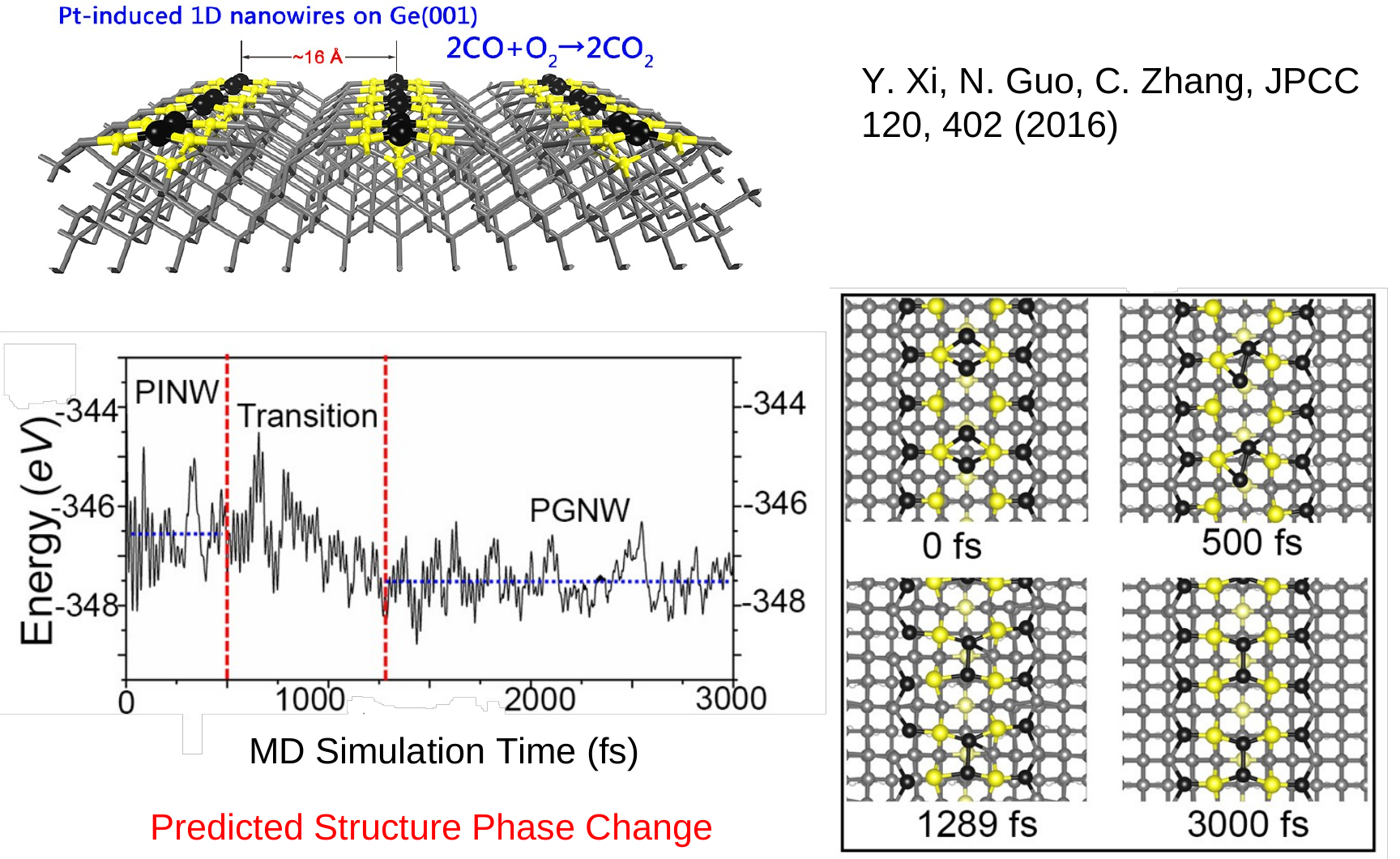
This surface also provides a setting for CO oxidation:

$$2\mathrm{CO}+\mathrm O_2\rightarrow2\mathrm{CO}_2.$$

The coordination environment determines which surface atoms bond to an adsorbed molecule, so reconstruction can also change catalytic activity. Xi, Guo & Zhang, 2016

Relating energy changes to structural changes

The horizontal axis of the energy trajectory is actual MD simulation time, measured in $\mathrm{fs}$. Since $1000\,\mathrm{fs}=1\,\mathrm{ps}$, the full trajectory covers about $3\,\mathrm{ps}$. The initial PINW structure vibrates around a higher energy level, enters the transition region between approximately $500$ and $1300\,\mathrm{fs}$, and then fluctuates around the lower level associated with PGNW.

Representative energies before and after the transition are approximately $-346.6$ and $-347.5\,\mathrm{eV}$, differing by about $0.9\,\mathrm{eV}$. This is the difference between the energy levels of the two stages. A reaction barrier is instead the energy rise from the initial state to the transition state along a path.

Snapshots at $0$, $500$, $1289$, and $3000\,\mathrm{fs}$ show positions and connections changing within the same local region, with a new wire arrangement retained at later times. Vibrations continue within each stage; the structural transformation is the change from one atomic arrangement to another.

In BO MD, each step first obtains the electronic ground-state energy of the current configuration, calculates forces from its gradient, and then advances the atoms. As atoms approach or separate, orbital overlap and coordination change, and new bonding takes the system into another low-energy region. The energy curve tells us when a change occurs; coordinates, bond lengths, and coordination tell us what changes.

Adsorption and surface reconstruction affect each other

As $\mathrm O_2$ approaches the Ge wire, Ge atoms can rearrange to form a new adsorption configuration. Xi, Guo & Zhang, 2016, Supporting Information

The molecule and surface jointly determine the potential energy surface. When adsorption creates new bonds, the original local equilibrium positions also change. Relaxing the relevant surface atoms together with the molecule gives the jointly stable structure of the adsorbate and reconstructed surface.

7. Self-tests

1. Does the BO approximation necessarily make the nuclei classical? No. BO first provides an electronic potential energy surface, on which the nuclei can still be treated quantum mechanically. Newtonian trajectories follow only after the additional classical-nuclei approximation.
2. Why does the Hellmann–Feynman formula hold when the electronic wavefunction changes with atomic position? For an exact normalized eigenstate, the wavefunction-derivative terms cancel through the eigenvalue equation and normalization. A finite, position-dependent basis requires Pulay corrections.
3. Which force is used in the final Velocity Verlet half step? The force at the new positions, $\mathbf F_i^{n+1}$, obtained after updating positions and recalculating the forces.
4. Are temperature fluctuations and a nonconstant system energy normal in NVT simulations? They can be. The system exchanges energy with the bath, and the equilibrium ensemble allows fluctuations. Check the averages, distributions, sampling, and integration stability.

V. Thermal Catalysis

1. From electronic energy to chemical reactions

At fixed atomic positions, first solve for the electronic ground state. After the atoms move, solve for the new ground state. Under the Born–Oppenheimer approximation, the electronic ground-state energy $E_e(\mathbf R)$ and the nuclear repulsion energy together define the potential energy surface on which the nuclei move:

$$E_{\mathrm{BO}}(\mathbf R)=E_e(\mathbf R)+V_{\mathrm{NN}}(\mathbf R).$$

The force on an atom is the negative gradient of the total potential energy with respect to its nuclear coordinates:

$$\mathbf F_I=-\nabla_I E_{\mathrm{BO}} =\mathbf F_I^{\mathrm{NN}}-\nabla_I E_e, \qquad M_I\ddot{\mathbf R}_I=\mathbf F_I.$$

$I$ labels an atom, $M_I$ is its mass, and $\mathbf F_I^{\mathrm{NN}}$ is the force due to nuclear repulsion. The minus sign makes the force point toward locally decreasing energy. Electronic self-consistency solves the electronic problem at the current nuclear coordinates; structural convergence additionally requires sufficiently small forces on the atoms that are allowed to move.

The same energies and forces serve different purposes. Structure optimization finds stable geometries; molecular dynamics advances positions and velocities in time using the atomic masses; reaction-path calculations search for a route across the barrier between two stable structures. Ordinary minimization stops in the reactant energy minimum, and short MD trajectories often miss rare barrier-crossing events. Dedicated path-search methods are therefore needed.

Thermal catalysis asks three questions: which bond must be activated, how the catalyst helps it rearrange, and how high a barrier the reaction must cross. Atomic positions reveal changes in bonding, while the energy profile gives their energetic cost. Together, they describe the reaction mechanism.

2. Why exothermic reactions still have barriers

The local minimum containing the reactants is the initial state (IS), and the product minimum is the final state (FS). The connecting path usually passes through a transition state (TS). The energy difference from the current reactant minimum to the TS is the activation barrier:

$$E_a=E_{\mathrm{TS}}-E_{\mathrm{IS}}.$$

Low product energy establishes only that the overall reaction releases energy. Before new bonds can form, the system often has to weaken existing bonds and rearrange its geometry, producing an energy maximum along the way. A reaction coordinate orders these configurations by reaction progress. It may be a bond length or distance along the path; it is not elapsed time.

The high-energy tail of the thermal distribution allows a small fraction of the ensemble to cross the barrier. Raising the temperature increases this fraction. A catalyst instead provides an alternative path with a lower barrier through adsorption, electron transfer, and intermediate formation. The available sites are regenerated after a complete catalytic cycle. For the same net reaction and thermodynamic initial and final states, the catalyst speeds up equilibration while leaving the reaction free energy and equilibrium constant unchanged.

The three types of catalysis differ in how the reaction is driven: thermocatalysis relies on thermal activation, electrocatalysis uses an applied potential to control electron transfer, and photocatalysis uses photoexcitation. This chapter focuses on thermally activated reactions.

3. $\mathrm{Fe}_2\mathrm C_{12}$: Donating electrons to oxygen antibonding orbitals

The activity of two-dimensional $\mathrm{Fe}_2\mathrm C_{12}$ comes from its exposed Fe sites. They donate electrons to the oxygen molecule's $2\pi^*$ antibonding orbitals, weakening the O–O bond and making oxygen more reactive toward CO. Each primitive cell contains two Fe atoms and twelve C atoms. Each Fe is coordinated to three C atoms, with Fe atoms protruding on opposite sides of the carbon plane. The carbon network anchors Fe and adjusts its electronic states through coordination, creating single-atom active sites. Li et al. (2021)

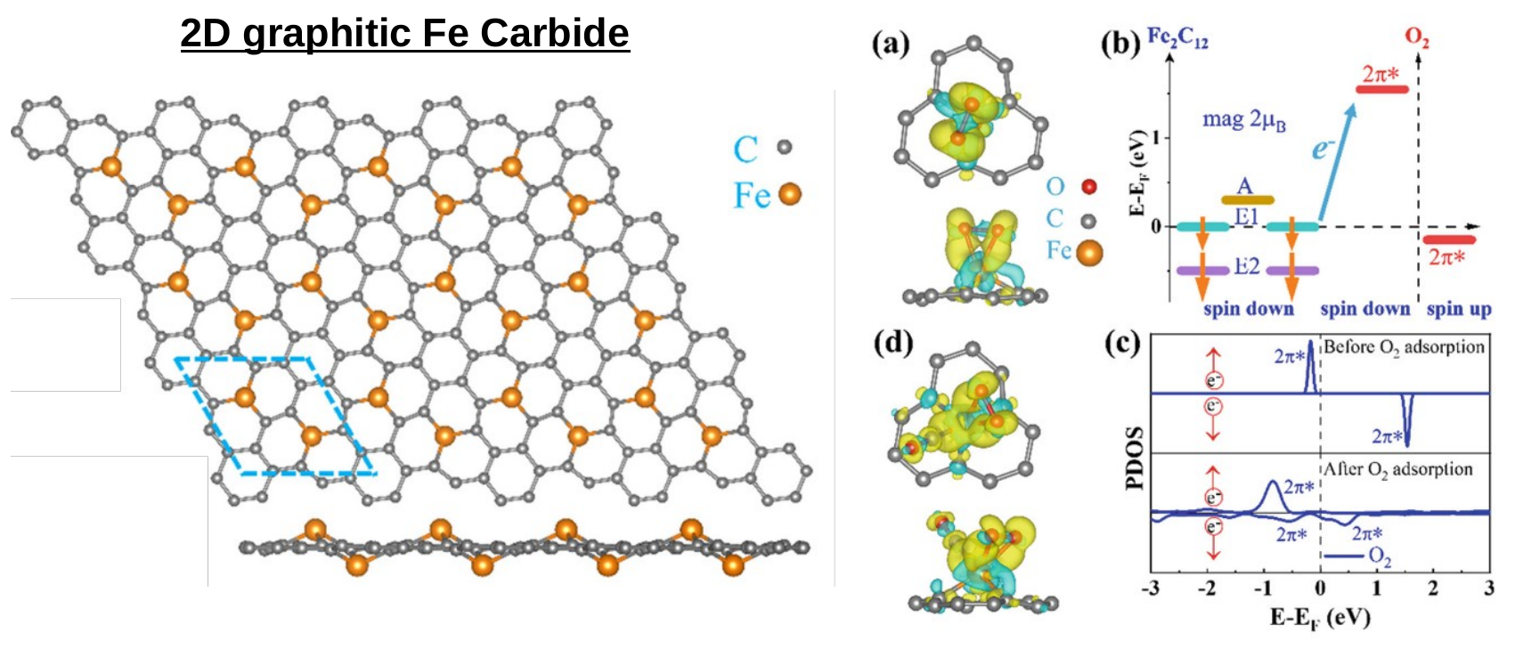
Fe sites donate electrons to oxygen antibonding states. In the charge-density difference isosurfaces, yellow indicates electron accumulation and cyan indicates depletion.

Why oxygen becomes activated

The Fe magnetic moment is approximately $1\mu_{\mathrm B}$ per atom and $2\mu_{\mathrm B}$ per primitive cell. Near the Fermi energy $E_{\mathrm F}$, the spin-down $E_1$ states are partially occupied and can donate electrons to empty oxygen antibonding states. After side-on adsorption, oxygen gains approximately $0.78|e|$. The O–O bond length increases from $1.23$ to $1.40\,\text{\AA}$, while the oxygen magnetic moment decreases from $2.0$ to $0.55\mu_{\mathrm B}$.

This electron transfer can be understood through the charge-density difference and the projected density of states (PDOS). The charge-density difference is defined as:

$$\Delta\rho(\mathbf r) =\rho_{\mathrm{combined}}(\mathbf r) -\rho_{\mathrm{catalyst}}(\mathbf r) -\rho_{\mathrm{adsorbate}}(\mathbf r).$$

The separated fragments and the combined system use the same atomic positions and computational settings. $\Delta\rho>0$ indicates local electron accumulation after adsorption, and $\Delta\rho<0$ indicates depletion.

The PDOS displays oxygen-related electronic states as a function of $E-E_{\mathrm F}$. Before adsorption, the spin-down $2\pi^*$ states are empty. After adsorption, some of these states move below the Fermi energy and become occupied. The additional antibonding electrons weaken the net bonding, lengthening O–O. Spin-resolved PDOS plots often place the two channels on opposite sides of zero; the downward-mirrored curve still represents a positive density of states.

One oxygen molecule oxidizes two CO molecules in sequence

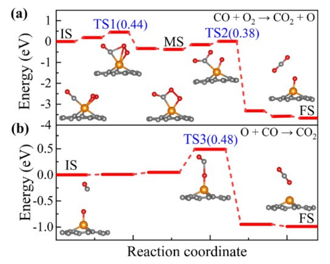
The first stage releases one carbon dioxide molecule and leaves adsorbed oxygen; the second removes the remaining oxygen. Each local barrier is measured from its preceding energy minimum.

CO and oxygen first coadsorb on Fe and then react through a Langmuir–Hinshelwood (LH) mechanism. They rearrange to form an OCOO intermediate, pass through the first transition state, and enter a metastable intermediate minimum (MS). O–O then stretches further and breaks through the second transition state, releasing the first carbon dioxide molecule:

$$\mathrm{CO}_{\mathrm{ads}}+\mathrm O_{2,\mathrm{ads}} \longrightarrow \mathrm{CO}_2+\mathrm O_{\mathrm{ads}}.$$

The vacuum path used for comparison in this example has a barrier of approximately $3\,\mathrm{eV}$. The catalytic path divides the reaction into more accessible steps, with the two local barriers equal to $0.44$ and $0.38\,\mathrm{eV}$. A second CO then reacts with the remaining adsorbed oxygen, crossing a barrier of $0.48\,\mathrm{eV}$:

$$\mathrm{CO}+\mathrm O_{\mathrm{ads}}\longrightarrow\mathrm{CO}_2.$$

Adding the two stages gives the net reaction:

$$2\mathrm{CO}+\mathrm O_2\longrightarrow2\mathrm{CO}_2.$$

The adsorption energy of $\mathrm{CO}_2$ on Fe is only approximately $-0.03\,\mathrm{eV}$, so the product binds weakly and can leave readily. The catalyst thus meets three requirements: it activates oxygen, provides low barriers for subsequent reactions, and allows product desorption to restore the site.

Each barrier is measured from its preceding energy minimum:

$$E_{a,1}=E_{\mathrm{TS}_1}-E_{\mathrm{IS}}, \qquad E_{a,2}=E_{\mathrm{TS}_2}-E_{\mathrm{MS}}.$$

For example, if MS lies at $-0.60\,\mathrm{eV}$ and the following TS lies at $-0.22\,\mathrm{eV}$, the local barrier is still $0.38\,\mathrm{eV}$. A later maximum below the original IS does not make the step from the current intermediate barrierless. When the two stages are plotted separately, each can use its own initial state as zero. Combining them into one energy profile requires a consistent reference for the adsorbates, gas-phase molecules, and catalyst.

For the Eley–Rideal (ER) mechanism, in which gas-phase CO directly attacks adsorbed oxygen, the first-stage barrier is $0.79\,\mathrm{eV}$. The coadsorbed LH first stage is therefore easier to cross. The rate of the complete cycle also depends on the populations of the adsorbed states and the kinetic prefactors. Li et al. (2021)

4. The Arrhenius relation: how barriers affect rates

A thermally activated rate can be understood as the attempt rate multiplied by the fraction of successful barrier crossings. For an energy barrier $E_a$ per reaction event, the Arrhenius equation is:

$$k=A\exp\!\left(-\frac{E_a}{k_{\mathrm B}T}\right).$$

$k$ is the rate constant, and $A$ is the pre-exponential factor, which includes the attempt frequency, orientation, and statistical factors. $A$ and $k$ have the same units, usually $\mathrm{s}^{-1}$ for a first-order reaction or a simple hopping process. The full reaction rate also includes reactant concentrations or surface coverages.

The exponent must be dimensionless. When $E_a$ is given per reaction event in eV, $k_{\mathrm B}$ must be in eV/K and $T$ in K. For a molar activation energy, use the gas constant $R$ instead:

$$k=A\exp\!\left(-\frac{E_{a,\mathrm{mol}}}{RT}\right).$$

For example, convert $50\,\mathrm{kJ\,mol^{-1}}$ to $50000\,\mathrm{J\,mol^{-1}}$ before combining it with $RT$ expressed in joule-based units.

Taking the logarithm gives:

$$\ln k=\ln A-\frac{E_a}{k_{\mathrm B}}\frac{1}{T}.$$

Over a temperature range in which the mechanism, $A$, and $E_a$ remain approximately constant, plotting $\ln k$ against $1/T$ gives a straight line with slope $-E_a/k_{\mathrm B}$. A slope of $-6000\,\mathrm K$ therefore gives $E_a\approx0.517\,\mathrm{eV}$.

To compare two paths at the same temperature:

$$\frac{k_2}{k_1} =\frac{A_2}{A_1} \exp\!\left(\frac{E_{a,1}-E_{a,2}}{k_{\mathrm B}T}\right).$$

Equal prefactors cancel. At $300\,\mathrm K$, $k_{\mathrm B}T\approx0.02585\,\mathrm{eV}$. Lowering the barrier from $0.50$ to $0.40\,\mathrm{eV}$ increases the rate constant by:

$$\frac{k_{\mathrm{new}}}{k_{\mathrm{old}}} =\exp\!\left(\frac{0.10}{0.02585}\right) \approx47.9.$$

For the same process at two temperatures, taking $A$ and $E_a$ as constant gives:

$$\ln\frac{k(T_2)}{k(T_1)} =\frac{E_a}{k_{\mathrm B}} \left(\frac{1}{T_1}-\frac{1}{T_2}\right).$$

Increasing the temperature makes the right-hand side positive, so the rate increases. DFT paths usually provide electronic energy differences. Quantitative finite-temperature rates may additionally require vibrational, entropic, and free-energy contributions.

5. Why metals are useful, and why adsorption must not be too strong

Metals have states near the Fermi energy that can donate or accept electrons. Upon contact with a reactant, these states hybridize with molecular orbitals, allowing existing bonds to weaken and new bonds to form. Electron transfer depends on energy alignment, occupation, and orbital overlap: a metal can donate to unoccupied or partially occupied molecular orbitals, while the molecule can also donate back to the metal.

For a finite cluster, the HOMO–LUMO gap is the energy difference between the highest occupied molecular orbital and the lowest unoccupied molecular orbital. Small Fe, Au, and Pt clusters have relatively small gaps and can often rearrange electrons at low energetic cost. Changing the atom count changes coordination and orbital splitting, so the gap can vary nonmonotonically with cluster size.

A small gap indicates that electrons can redistribute relatively easily. Catalysis also requires effective coupling to the target reactant and suitable binding strengths. Ligands that constrain Co coordination, or a carbon network that embeds metal atoms, can adjust orbital splitting, reactant approach directions, and binding through the surrounding atoms and bond angles.

The Sabatier principle requires binding that is neither too weak nor too strong. Weak reactant adsorption gives low coverage and makes effective electron transfer difficult. Strongly bound intermediates or products can occupy sites for long periods. A complete cycle must accommodate adsorption, bond formation and breaking, and product desorption.

Energetically, lowering only an intermediate minimum can slow the following reaction. If an intermediate falls from $-0.2$ to $-1.2\,\mathrm{eV}$ while the next TS remains at $0\,\mathrm{eV}$, the local barrier increases from $0.2$ to $1.2\,\mathrm{eV}$. A catalyst must be assessed using the height of each subsequent TS above its preceding intermediate, rather than by seeking ever more negative adsorption energies.

6. $\mathrm{Au}_{20}/\mathrm{CeO}_2$: Active sites can form during the reaction

On a ceria-supported gold cluster, CO can pull a low-coordination Au atom into a mobile Au–CO unit, bringing CO close to lattice oxygen. Ceria supplies oxygen, the Au atom leaves and returns to the cluster, and product desorption helps regenerate the site. This calculated pathway dynamically forms a single-atom active site. Wang et al. (2015)

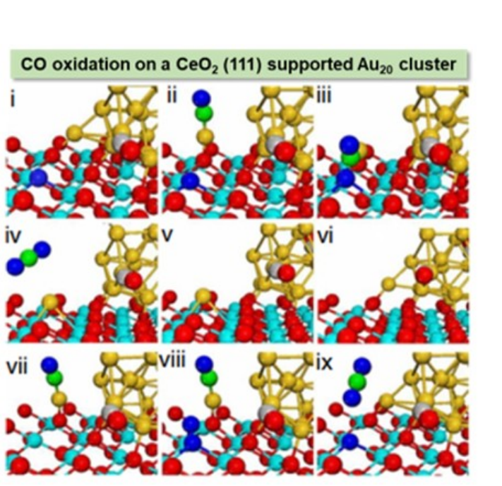
CO helps Au leave the cluster and react with lattice oxygen. After Au returns, gas-phase oxygen replenishes the vacancy and regenerates the site.

The cycle begins with CO binding to Au at the cluster edge. The Au–CO unit leaves the edge and moves toward the support. CO then attacks lattice oxygen, forming a bent carbon–oxygen intermediate. Desorption of the first $\mathrm{CO}_2$ molecule leaves an oxygen vacancy in the support, where Au temporarily resides.

Au then returns to the cluster, exposing the oxygen vacancy again. A second CO forms a new Au–CO unit, while $\mathrm O_2$ adsorbs at the vacancy and forms a peroxo species. After the second CO is oxidized, Au returns to the cluster and the remaining O fills the lattice vacancy. The support supplies lattice oxygen and is subsequently replenished by gas-phase oxygen, the defining feature of a Mars–van Krevelen mechanism.

The mobile Au–CO site facilitates product release: desorbing the first $\mathrm{CO}_2$ molecule costs $0.27\,\mathrm{eV}$, compared with $1.29\,\mathrm{eV}$ for the corresponding path reacting at a cluster site. The barrier for Au to return from the oxygen vacancy to the cluster is $0.89\,\mathrm{eV}$, making this the rate-limiting step of the calculated path. A desorption energy difference and a barrier to crossing a TS describe distinct processes. Wang et al. (2015)

Catalyst regeneration means restoring a usable site after a complete cycle. Atomic migration, coordination changes, and electron transfer can all be part of that cycle.

7. Saddle points and reaction energies on a potential energy surface

A minimum energy path (MEP) connects the relevant local minima. Perpendicular to the path, the energy has been locally minimized; along the path, it can still rise or fall. An arbitrary connecting curve may pass over higher slopes, so the chosen path directly affects the barrier.

The forward barrier, reaction energy, and reverse barrier are:

$$E_a^{\mathrm{fwd}}=E_{\mathrm{TS}}-E_{\mathrm{IS}}, \qquad \Delta E=E_{\mathrm{FS}}-E_{\mathrm{IS}},$$

$$E_a^{\mathrm{rev}} =E_{\mathrm{TS}}-E_{\mathrm{FS}} =E_a^{\mathrm{fwd}}-\Delta E.$$

An exothermic reaction satisfies $\Delta E<0$, so the reverse barrier through the same saddle point is higher. Adding the same constant to all energies leaves these differences unchanged. For example, with $E_{\mathrm{IS}}=-10.0$, $E_{\mathrm{TS}}=-9.4$, and $E_{\mathrm{FS}}=-10.8\,\mathrm{eV}$, the forward barrier is $0.6\,\mathrm{eV}$, the reaction energy is $-0.8\,\mathrm{eV}$, and the reverse barrier is $1.4\,\mathrm{eV}$.

A TS is a first-order saddle point. It first satisfies the stationarity condition in all relevant coordinates:

$$\nabla E(\mathbf R_{\mathrm{TS}})=0.$$

The Hessian matrix then describes the local curvature:

$$H_{ab}=\frac{\partial^2E}{\partial R_a\partial R_b}.$$

The curvature is negative along one internal direction and positive along the others. One negative eigenvalue of the mass-weighted Hessian corresponds to an imaginary frequency, whose mode should follow the intended reaction direction. Translational, rotational, and other zero modes are treated separately. Descending in both directions along the unstable mode tests whether the saddle connects the intended reactant and product.

8. Constrained scans and gold clusters supported on thin MgO

Fixing one reaction coordinate

Constrained energy minimization is useful when the main geometric change is clear. For example, progressively shorten a forming C–O bond while relaxing the other coordinates that are allowed to move.

Start from the optimized initial state, fix the reaction coordinate $q$, and perform electronic self-consistency and constrained structural optimization. Then change $q$ by a small amount and use the preceding structure as the next initial guess. This produces a relaxed energy scan:

$$E_{\mathrm{rel}}(q) =\min_{\mathbf R:\,Q(\mathbf R)=q}E(\mathbf R).$$

$Q(\mathbf R)$ extracts the selected coordinate from the full atomic configuration. In practice, the optimization generally finds a local minimum on the constraint surface. Using the initial state $q_a$ as the reference:

$$\Delta E(q)=E_{\mathrm{rel}}(q)-E_{\mathrm{rel}}(q_a).$$

Check structural continuity during the scan and use smaller steps near the maximum. If the reaction involves substantial rotation, sideways motion, or several bonds changing together, add coordinates or optimize the whole path. Forward and reverse scans can also help identify different branches of local structures.

The scan maximum is an initial guess for the TS. Refine the stationary point in all relevant degrees of freedom, check for one reaction-related imaginary frequency, and descend along both directions of that mode to establish whether the constrained-path maximum is a true transition state.

Why $\mathrm{Au}_{20}$/MgO/Mo has a low barrier

The Mo substrate supplies electrons through two thin MgO layers to the two-dimensional $\mathrm{Au}_{20}$ interface. These electrons enter the $2\pi^*$ antibonding states of adsorbed oxygen and lengthen O–O. CO on a neighboring MgO site can then react with it over a low barrier. The gold-cluster interface anchors and activates oxygen, while the MgO site allows CO to approach from a suitable direction. Zhang, Yoon & Landman (2007)

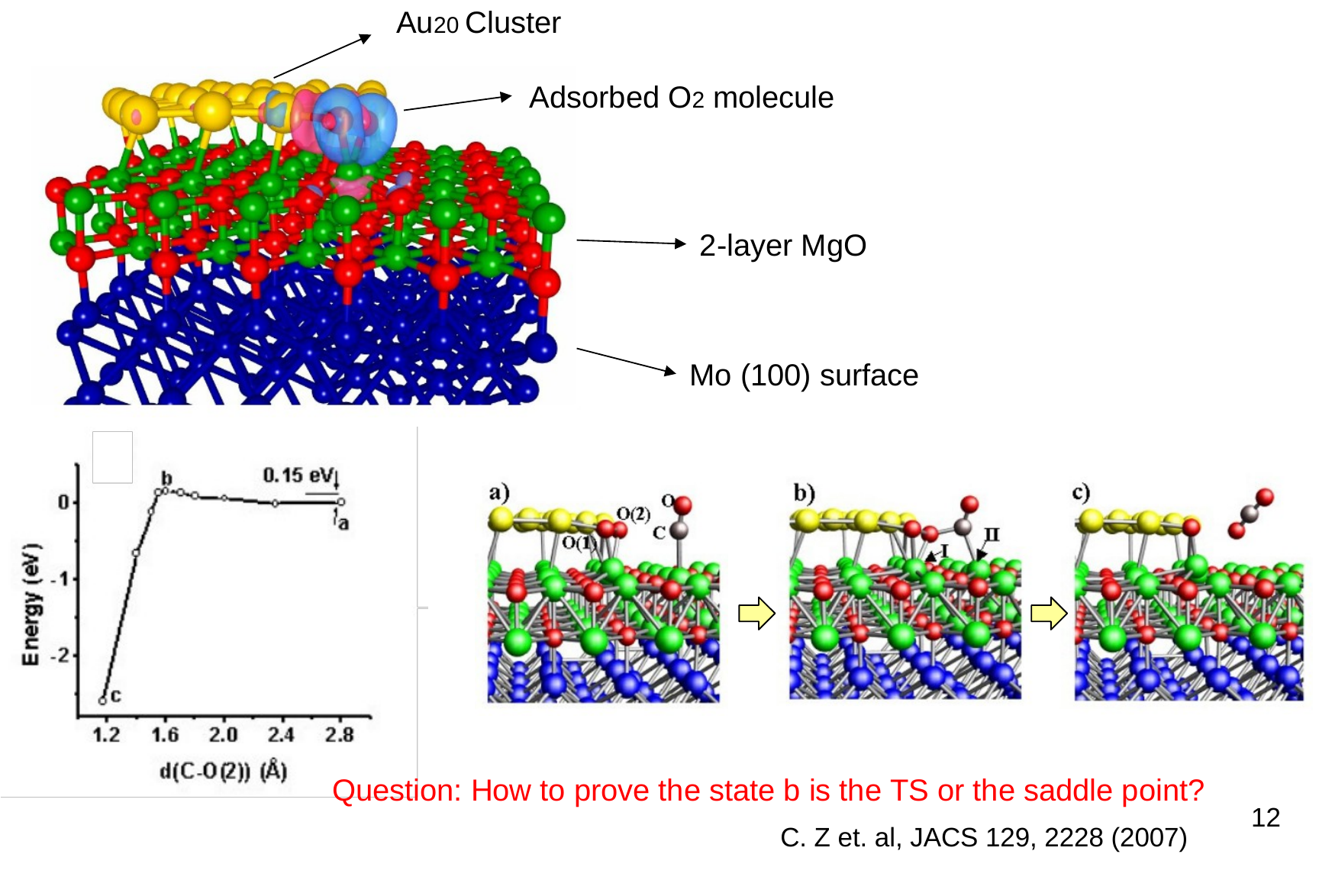
Mo supplies electrons through thin MgO to the gold-cluster interface. As the C–O distance decreases, the system crosses a maximum of approximately $0.15\,\mathrm{eV}$ and forms carbon dioxide.

This LH path starts from configuration $a$, in which CO and oxygen are coadsorbed. The scan coordinate is the distance from the C atom in CO to the nearest O atom in the oxygen molecule:

$$q=d(\mathrm C,\mathrm O^{(2)}).$$

The C–O distance starts at $2.85\,\text{\AA}$ in the initial state. In configuration $b$ near the maximum, it has shortened to $1.60\,\text{\AA}$, while O–O has lengthened from $1.52$ to $1.55\,\text{\AA}$. After the new C–O bond forms, $\mathrm{CO}_2$ leaves the surface. Relative to the coadsorbed initial state, the barrier along this path is approximately:

$$E^\ddagger=E(b)-E(a)\simeq0.15\,\mathrm{eV}.$$

If the horizontal axis is the C–O distance itself, the reaction proceeds toward decreasing distance. The peak height measures the barrier, while the subsequent energy decrease represents the energy released in product formation.

The adsorption site of CO changes the path. CO adsorbed at the Au edge gives a barrier of approximately $1.0\,\mathrm{eV}$; an ER path in which gas-phase CO directly attacks adsorbed oxygen has a barrier of approximately $0.2\,\mathrm{eV}$. The low barrier combines electronic and geometric effects: oxygen first gains antibonding electrons, and CO then approaches the activated oxygen from a neighboring MgO site. Zhang, Yoon & Landman (2007), Supporting Information

9. Self-tests

Why can a reaction be slow even when its products have much lower energy?

Reaction energy compares the initial and final states; the rate depends on the local barrier from the current minimum to the TS. Stabilizing products and lowering the transition state are different changes.

How can you assess whether a catalyst can sustain repeated turnover?

It must activate reactants and lower key barriers, but also convert residual intermediates, release products, and regenerate sites. Strong adsorption alone does not guarantee a high turnover rate.

VI. Nudged Elastic Band Method

1. From one reaction coordinate to a chain of configurations

A single bond length describes some reactions clearly, but molecular rotation, concerted changes in several bonds, or surface reconstruction often require more coordinates. NEB (nudged elastic band) starts from known initial and final states and directly optimizes a chain of complete configurations, allowing the whole chain to bend toward a low-energy channel.

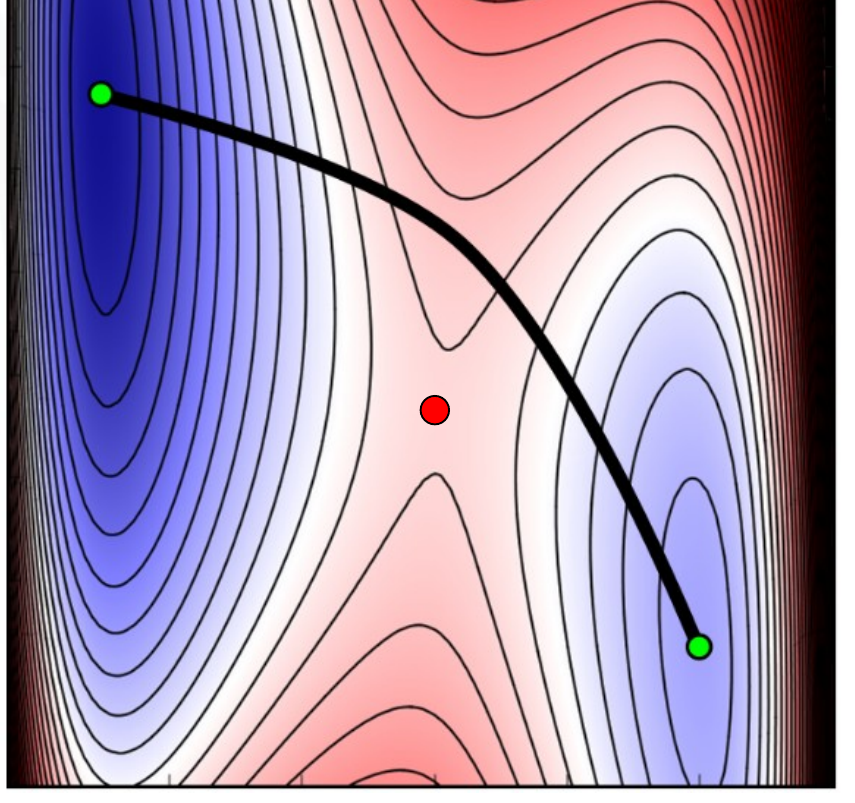
The endpoints lie in two energy minima. The initial path must adjust in configuration space to pass through the low-energy channel connecting them.

A configuration of $N$ atoms is written as:

$$\mathbf R=(x_1,y_1,z_1,\ldots,x_N,y_N,z_N), \qquad E=E(\mathbf R).$$

An image consists of the complete atomic coordinates and the corresponding potential energy and forces. A two-dimensional contour plot is only a schematic of the high-dimensional potential energy surface (PES): each point represents the entire atomic system. Fixing some substrate atoms reduces the number of degrees of freedom that can be optimized.

Each iteration first solves the electronic problem at the corresponding geometry. Magnetic systems also require tracking the electronic spin state and using consistent spin treatment across all images. The nuclear path is optimized on the selected electronic potential energy surface; transitions between different spin surfaces require a nonadiabatic treatment.

Discretize the path as:

$$\mathbf R_0,\mathbf R_1,\ldots,\mathbf R_{M-1},\mathbf R_M.$$

There are $M+1$ images. $\mathbf R_0$ and $\mathbf R_M$ are the optimized IS and FS and are usually fixed, while the intermediate images are optimized together. The distances between neighboring configurations are:

$$d_i^+=|\mathbf R_{i+1}-\mathbf R_i|, \qquad d_i^-=|\mathbf R_i-\mathbf R_{i-1}|.$$

With a Cartesian metric, square and sum all displacement components of corresponding atoms, then take the square root. All images must therefore share consistent atom counts, element ordering, atom correspondence, and cell descriptions.

More images resolve curved paths, intermediate minima, and variations near the maximum, at the cost of more electronic-structure calculations. Usually, first establish a clear channel, then increase sampling where the path changes rapidly. The energies can be plotted against cumulative configuration-space distance after optimization; this measures reaction progress, not elapsed time.

2. Why NEB projects the forces

If each intermediate configuration is minimized independently, the images fall into energy minima and leave the barrier region unsampled. Ordinary connecting springs can instead straighten a curved path to shorten the band, causing corner cutting. NEB separates the two tasks: the physical force moves the path perpendicular to its tangent toward the valley, while the spring force distributes images along the path.

Tangential and perpendicular components of the physical force

The physical force on image $i$ is:

$$\mathbf F_i^{\mathrm{phys}}=-\nabla E(\mathbf R_i).$$

Let $\boldsymbol\tau_i$ be a unit tangent estimated from neighboring configurations, satisfying $\boldsymbol\tau_i\cdot\boldsymbol\tau_i=1$. The projection of the physical force along the path is:

$$\mathbf F_{i,\parallel}^{\mathrm{phys}} =(\mathbf F_i^{\mathrm{phys}}\cdot\boldsymbol\tau_i)\boldsymbol\tau_i.$$

The dot product gives the scalar tangential component. Multiplying by the unit tangent gives its vector projection. Subtracting this projection leaves the perpendicular component:

$$\mathbf F_{i,\perp}^{\mathrm{phys}} =\mathbf F_i^{\mathrm{phys}} -(\mathbf F_i^{\mathrm{phys}}\cdot\boldsymbol\tau_i)\boldsymbol\tau_i.$$

It satisfies $\mathbf F_{i,\perp}^{\mathrm{phys}}\cdot\boldsymbol\tau_i=0$. Normalize the tangent before applying these formulas directly.

The physical tangential force would push images toward the energy minima, so ordinary NEB removes it. The retained perpendicular force lets the path move down the valley walls toward the MEP. A converged MEP satisfies:

$$\mathbf F_\perp^{\mathrm{phys}}=\mathbf 0.$$

A tangential downhill force can still exist along the MEP. The complete physical force vanishes only at the TS or another stationary point.

Retaining only the tangential spring force

With a uniform spring constant $k$, the tangential spring force is:

$$\mathbf F_{i,\parallel}^{\mathrm{spring}} =k(d_i^+-d_i^-)\boldsymbol\tau_i.$$

When the forward spacing is larger, the spring pulls the image along $+\boldsymbol\tau_i$. Tangential balance makes the forward and backward spacings equal. The perpendicular spring component is removed so that it does not straighten a curved channel.

The effective force used for optimization is therefore:

$$\mathbf F_i^{\mathrm{NEB}} =\mathbf F_{i,\perp}^{\mathrm{phys}} +\mathbf F_{i,\parallel}^{\mathrm{spring}}.$$

$k$ can be expressed in $\mathrm{eV}\,\text{\AA}^{-2}$. Multiplying by a configuration-space distance gives force units of $\mathrm{eV}\,\text{\AA}^{-1}$.

For example, take $\boldsymbol\tau=(1,0)$ and $\mathbf F^{\mathrm{phys}}=(2,-3)\,\mathrm{eV}\,\text{\AA}^{-1}$, forward and backward spacings of $2$ and $1\,\text{\AA}$, and $k=1.5\,\mathrm{eV}\,\text{\AA}^{-2}$. The perpendicular physical force is $(0,-3)$ and the spring force is $(1.5,0)$, giving:

$$\mathbf F^{\mathrm{NEB}}=(1.5,-3)\,\mathrm{eV}\,\text{\AA}^{-1}.$$

$\mathbf F_i^{\mathrm{NEB}}=0$ means that the perpendicular physical force vanishes and the tangential spring forces balance. The removed physical tangential force can remain nonzero, so an ordinary converged image can lie on a slope of the MEP.

3. Variable spring constants: denser sampling at high energy

Accurate peak energies require denser sampling near the saddle point. Increasing the spring constants in high-energy regions concentrates the available images in these segments.

Let $k_i$ connect images $i-1$ and $i$, and define:

$$E_{\mathrm{ref}}=\max(E_{\mathrm{IS}},E_{\mathrm{FS}}), \qquad \widetilde E_i=\max(E_{i-1},E_i),$$

$$\Delta k=k_{\max}-k_{\min}.$$

$E_{\max}$ is the highest physical energy on the current band. Assign each segment's spring constant using the higher energy of its two endpoints:

$$k_i= \begin{cases} k_{\max}-\Delta k\,\dfrac{E_{\max}-\widetilde E_i}{E_{\max}-E_{\mathrm{ref}}}, &\widetilde E_i>E_{\mathrm{ref}},\\[6pt] k_{\min},&\widetilde E_i\leq E_{\mathrm{ref}}. \end{cases}$$

When $\widetilde E_i=E_{\max}$, the segment uses the stiffest spring, $k_{\max}$. As its energy decreases to $E_{\mathrm{ref}}$, the constant returns continuously to $k_{\min}$. If $E_{\max}=E_{\mathrm{ref}}$, use constant springs to avoid a zero denominator.

When the forward and backward spring constants differ, the tangential force is:

$$\mathbf F_{i,\parallel}^{\mathrm{spring}} =(k_{i+1}d_i^+-k_i d_i^-)\boldsymbol\tau_i.$$

Tangential equilibrium requires equal tensions on the two sides:

$$k_{i+1}d_i^+\approx k_i d_i^-.$$

At the same tension, a larger $k$ gives a smaller spacing, so more images gather in high-energy regions. These springs control numerical sampling; they leave the physical potential energy unchanged.

For example, with $E_{\mathrm{ref}}=0$, $E_{\max}=0.8\,\mathrm{eV}$, $k_{\min}=1$, and $k_{\max}=5\,\mathrm{eV}\,\text{\AA}^{-2}$, a segment at $\widetilde E_i=0.6\,\mathrm{eV}$ has:

$$k_i=5-4\frac{0.8-0.6}{0.8} =4\,\mathrm{eV}\,\text{\AA}^{-2}.$$

4. Climbing Image NEB: moving directly toward a saddle point

The highest sampled image in ordinary NEB may lie on one side of the maximum. CI-NEB selects an image and drives it uphill along the path and downhill perpendicular to the path, directly toward the saddle point.

The physical force decomposes as $\mathbf F_\perp+\mathbf F_\parallel$. Retaining the perpendicular component and reversing the tangential component gives the target force $\mathbf F_\perp-\mathbf F_\parallel$. This is equivalent to subtracting twice the tangential component from the physical force:

$$\mathbf F^{\mathrm{CI}} =\mathbf F^{\mathrm{phys}} -2(\mathbf F^{\mathrm{phys}}\cdot\boldsymbol\tau)\boldsymbol\tau.$$

Substituting $\mathbf F^{\mathrm{phys}}=-\nabla E$ gives:

$$\mathbf F^{\mathrm{CI}} =-\nabla E+2(\nabla E\cdot\boldsymbol\tau)\boldsymbol\tau.$$

First obtain a reasonable channel with ordinary NEB. Then select the highest-energy intermediate image as the climbing image and remove its spring force. It can then reach the maximum without being constrained by equal spacing. The other images continue to use ordinary NEB forces and provide the path shape and local tangent.

Using the same example with $\boldsymbol\tau=(1,0)$ and $\mathbf F^{\mathrm{phys}}=(2,-3)$:

$$\mathbf F^{\mathrm{CI}} =(2,-3)-2(2,0)=(-2,-3).$$

The tangential component reverses sign, the perpendicular component stays unchanged, and no spring force is added.

The tangential and perpendicular directions are orthogonal, so $\mathbf F^{\mathrm{CI}}=0$ requires both components of the physical force to vanish, giving a physical stationary point. Check for one reaction-related negative-curvature mode and verify the initial and final states reached by descending in both directions along that mode to identify the intended TS.

Barrier accuracy has two aspects: whether the path has found the intended channel, and whether sampling near the maximum is sufficient. Different initial guesses for competing mechanisms address the first; more images and CI refinement address the second.

5. Constructing and optimizing the initial path

The simplest initial path is generated by linear interpolation:

$$\mathbf R_i^{(0)} =\left(1-\frac{i}{M}\right)\mathbf R_{\mathrm{IS}} +\frac{i}{M}\mathbf R_{\mathrm{FS}}, \qquad i=0,\ldots,M.$$

Every coordinate is interpolated with weight $i/M$, so the initial images are equally spaced in Cartesian configuration space. Their energy spacing depends on the potential energy surface. The endpoints should use consistent cells, atom numbering, constraints, electronic states, and computational accuracy.

For an atom moving from $(0,0)$ to $(2,1)\,\text{\AA}$ with five images in total, $M=4$. The three internal initial guesses are $(0.5,0.25)$, $(1,0.5)$, and $(1.5,0.75)\,\text{\AA}$. A many-atom system interpolates all coordinates simultaneously.

Inspect each interpolated geometry. Linear interpolation can make two exchanging atoms coincide, or compress internal bonds when a molecule rotates substantially. Add physically reasonable intermediate configurations or interpolate in segments when needed. With periodic boundaries, first unwrap coordinates onto a continuous branch consistent with the intended hop, then generate the path.

The NEB optimization proceeds as follows:

1. Calculate the electronic energy and physical atomic forces for each image.
2. Estimate and normalize the tangent from neighboring configurations.
3. Combine the perpendicular physical force with the tangential spring force and update the intermediate configurations.
4. Once the path is stable, activate the climbing image and refine the saddle point.
5. Check electronic self-consistency, converged forces, structural continuity, and sampling near the maximum. Extract the barrier from the energy difference between the relevant IS and TS.

6. Surface diffusion as a path-search problem

Chemical reactions connect structures with different bonding, while surface diffusion connects different adsorption positions. Both are transitions between minima on a potential energy surface, so both can be studied with NEB.

Diffusion may involve molecular rotation, coordination changes, and surface relaxation. The energy difference from the starting adsorption site to the CI-NEB saddle point is the barrier for that hop. A simple hopping model is:

$$\Gamma=\nu\exp\!\left(-\frac{E_{\mathrm{diff}}}{k_{\mathrm B}T}\right).$$

$\Gamma$ is the hopping rate, $\nu$ the attempt frequency, and $E_{\mathrm{diff}}$ the diffusion barrier. If the endpoints have different energies, the reverse barrier through the same saddle satisfies:

$$E_a^{\mathrm{rev}}=E_a^{\mathrm{fwd}}-\Delta E.$$

A deeper adsorption site requires more energy to escape. Equal endpoint energies imply equal forward and reverse barriers, but a high maximum can still lie between them. Obtaining a macroscopic diffusion coefficient from a single-hop rate also requires the hop distance, spatial dimension, accessible neighbors, and correlations between hops.

7. Graphene/Ru: from substrate defects to two-step CO oxidation

Local defects in the Ru surface weaken bonding between Ru and the carbon atoms above them, making those carbon atoms more able to donate electrons to adsorbed oxygen. Occupation of oxygen antibonding states lengthens O–O. Oxygen then reacts with gas-phase CO over relatively low barriers to form carbon dioxide. Guo, Yam & Zhang (2018)

Two substrate defects are considered: IA denotes a substitutional impurity atom replacing a surface Ru atom, and V denotes a single vacancy in the surface Ru layer. The active region lies in the graphene directly above the defect, where oxygen adsorbs on carbon atoms.

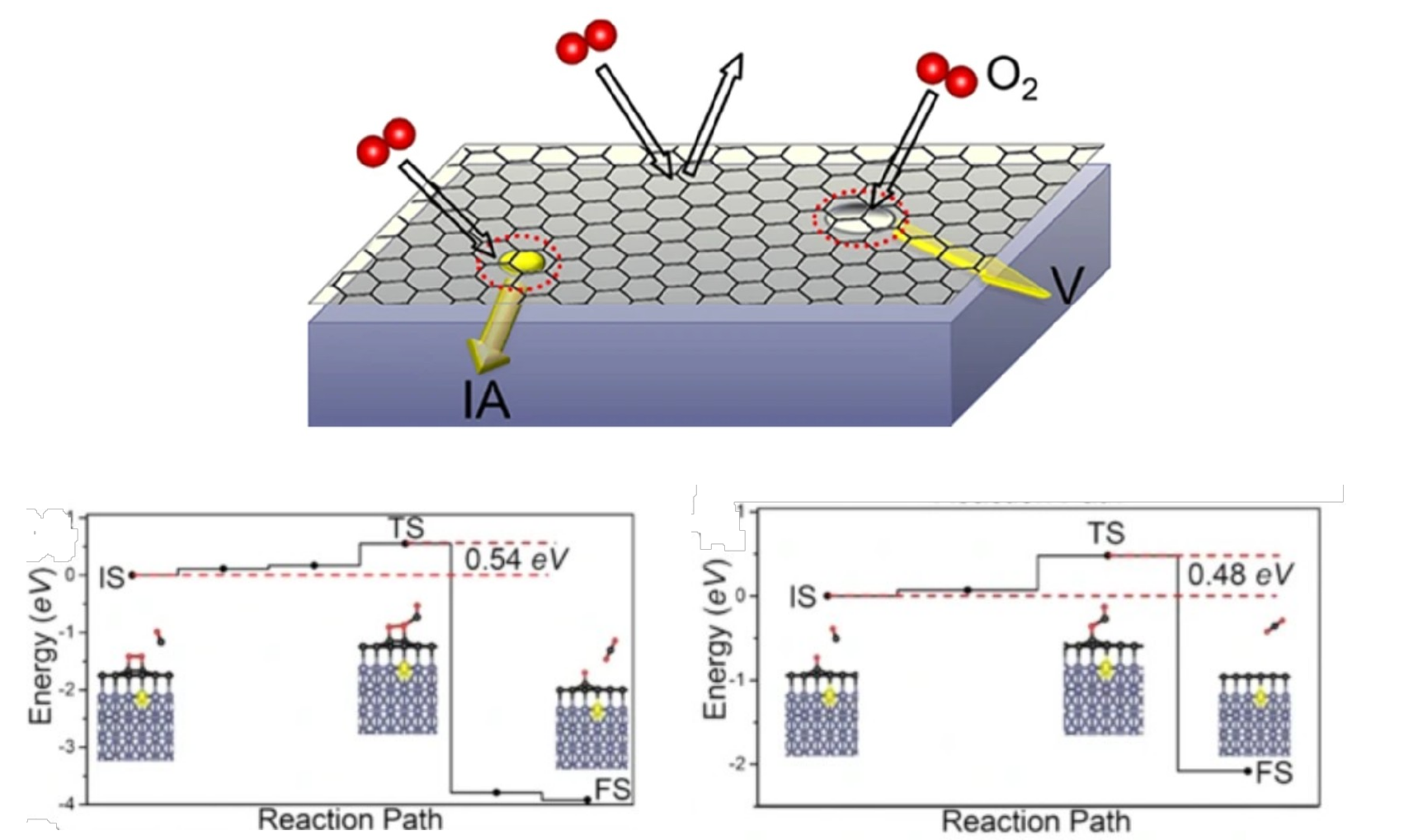
IA and V denote two substrate-defect types. The two energy profiles below describe consecutive oxidation steps in the same Au-substitution model, with barriers of $0.54$ and $0.48\,\mathrm{eV}$.

The specific two-step reaction uses the same Au-substituted Ru(0001) model, with graphene in the fcc-top registry. Au weakens nearby C–Ru bonding; upon oxygen adsorption, electrons enter the oxygen $2\pi^*$ antibonding states. Oxygen gains approximately $0.99|e|$, O–O lengthens from $1.23$ to $1.48\,\text{\AA}$, and the adsorption energy is $-0.43\,\mathrm{eV}$.

Gas-phase CO reacts with adsorbed oxygen through an Eley–Rideal (ER) mechanism. Near the first TS, O–O stretches while a new C–O bond forms. The first $\mathrm{CO}_2$ molecule is released, leaving one adsorbed oxygen atom:

$$\mathrm{CO}_{\mathrm{gas}}+\mathrm O_{2,\mathrm{ads}} \longrightarrow\mathrm{CO}_2+\mathrm O_{\mathrm{ads}}, \qquad E_{a,1}=0.54\,\mathrm{eV}.$$

A second CO removes the remaining oxygen, forming another carbon dioxide molecule:

$$\mathrm{CO}_{\mathrm{gas}}+\mathrm O_{\mathrm{ads}} \longrightarrow\mathrm{CO}_2, \qquad E_{a,2}=0.48\,\mathrm{eV}.$$

These barriers belong to consecutive steps in the same Au system, each measured from its own initial state to its CI-NEB saddle point. After the second step, the graphene site can accept another oxygen molecule and begin the next cycle. Guo, Yam & Zhang (2018)

The rate constant of each step can be understood using a thermally activated form:

$$k_i\simeq A_i\exp\!\left(-\frac{E_{a,i}}{k_{\mathrm B}T}\right).$$

The first step requires adsorbed oxygen molecules, whereas the second requires the remaining oxygen atoms. Their coverages depend on adsorption and the preceding reactions. Identifying the rate-determining step therefore requires both the local rate constants and these surface populations. Electron transfer explains oxygen activation, CI-NEB describes barrier crossing, and the complete cycle explains sustained site turnover.

8. Self-tests

Does zero ordinary NEB force imply zero physical atomic force?

Ordinary NEB requires only a vanishing perpendicular physical force and balanced tangential spring forces; a physical tangential force may remain. The climbing image reverses the physical tangential force, so its effective force vanishes only when both tangential and perpendicular physical forces vanish.

Why do variable springs increase the density of images at high energy?

At equilibrium, neighboring springs have equal tension. High-energy regions use larger spring constants, giving smaller spacings at the same tension and therefore denser sampling.

References

• Chuanhao Yao et al. Atomically-precise dopant-controlled single cluster catalysis for electrochemical nitrogen reduction. Nature Communications 11, 4389 (2020).
• Hao Wang et al. Structure phase change induced by nonequilibrium effects in molecular-scale junctions. Physical Review B 110, L121405 (2024). Author manuscript.
• Yongjie Xi; Na Guo; Chun Zhang. Predicted Unusual Catalytic Activity of One-Dimensional Pt-Induced Atomic Nanowires on Ge(001) Surface. The Journal of Physical Chemistry C 120(1), 402–406 (2016). Supporting Information.
• Danny E. P. Vanpoucke; Geert Brocks. Formation of Pt-induced Ge atomic nanowires on Pt/Ge(001): A density functional theory study. Physical Review B 77, 241308(R) (2008).
• Shulong Li et al. Highly stable two-dimensional metal-carbon monolayer with interpenetrating honeycomb structures. npj 2D Materials and Applications 5, 52 (2021).
• Yang-Gang Wang et al. Dynamic formation of single-atom catalytic active sites on ceria-supported gold nanoparticles. Nature Communications 6, 6511 (2015).
• Chun Zhang; Bokwon Yoon; Uzi Landman. Predicted Oxidation of CO Catalyzed by Au Nanoclusters on a Thin Defect-Free MgO Film Supported on a Mo(100) Surface. Journal of the American Chemical Society 129(8), 2228–2229 (2007). Supporting Information.
• Na Guo; Kah Meng Yam; Chun Zhang. Substrate engineering of graphene reactivity: towards high-performance graphene-based catalysts. npj 2D Materials and Applications 2, 1 (2018).